5 Statistical Inference
In Chapters 1-4, we learned how to describe patterns in our data. In this chapter, we introduce a category of statistical tools used for something more ambitious. Inferential statistics allow us to use patterns in our data to draw conclusions about things not directly appearing in our dataset. For example, we might try to answer questions about a counterfactual: what outcomes would we see for participants in a program if they had instead not participated? Or we might try to answer questions about a broader set of data to which we do not have access: based on the 100 clients who responded to my satisfaction survey, what can I conclude about satisfaction among all clients of my organization?
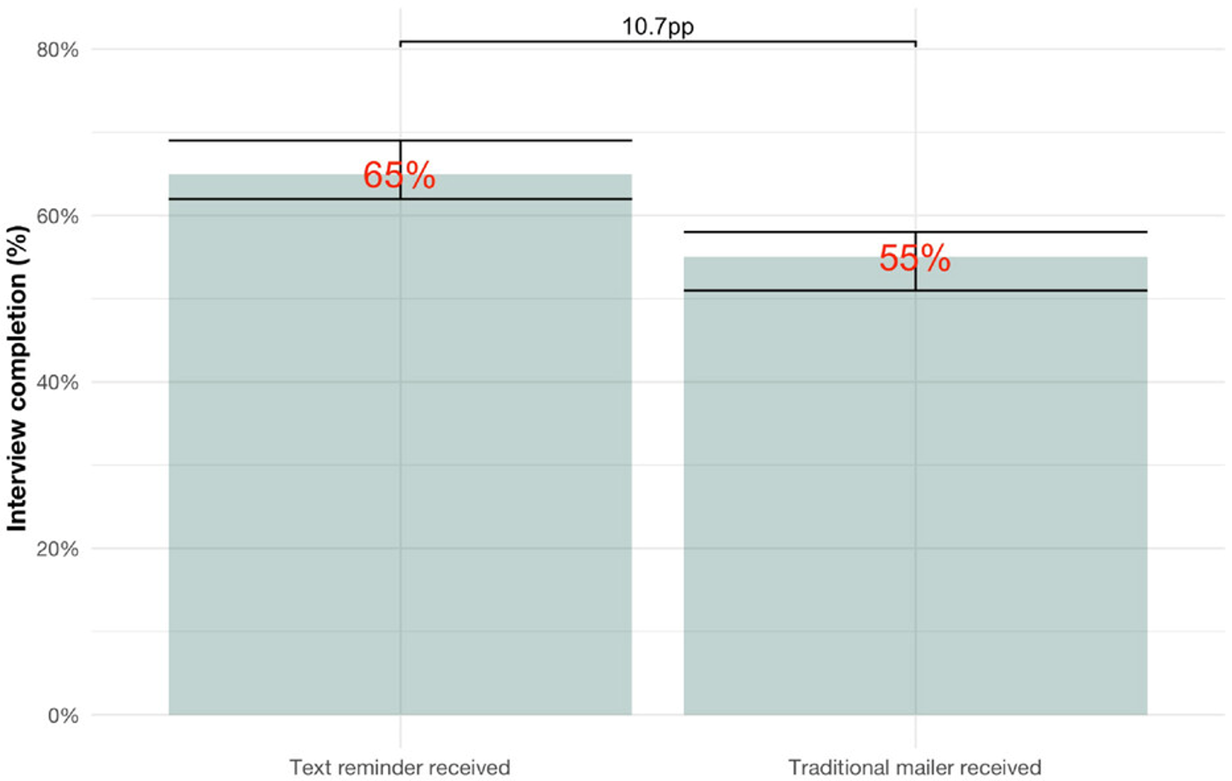
Kim et. al (2025) study the experience of people trying to access food assistance benefits in the U.S. One requirement of the assistance program is to complete an interview. Working together with a nonprofit organization and a local government, the researchers designed an experiment to study whether interview completion rates could be improved by sending text messages to remind applicants of upcoming appointments and inform them of a new drop-in interview option.
For the experiment, some study participants were assigned to be part of a control group and thus received only a traditional mailer and no text reminders. A control group refers to a set of participants who receive no intervention, helping to establish a baseline. The rest of the participants received the treatment, meaning the intervention of interest to researchers. In this case, the treatment consisted of text reminders that were sent in addition to the mailer. Assignment to treatment and control groups was based on each participant’s randomly-assigned case number: odd case numbers received the treatment while even case numbers received the control.
Using inferential statistics, the authors estimate how the text reminders affect the chances of completing an interview. The exact effect may vary depending on the study participant. We can game this out by imagining several distinct categories of applicants. Some applicants receiving the reminders would have completed the interview anyway, so for them the reminders had no effect. For others, the reminders were pivotal, causing them to attend an interview instead of missing it. And some missed the interview even with reminders (and possibly some because of the reminders, but I assume this is unlikely). Among those who did not receive the reminders, there were those who completed the interview anyway and for whom the reminders presumably would have had no effect (unless reminders somehow discouraged completion of the interview). There were also those who did not complete the interview but would have had they received the texts. Finally, there are those who did not complete the interview and wouldn’t have even with reminders.
In a perfect world, we might like to know whether and how the text reminders would have changed the behavior of each person in the study. This is impossible to determine, however, since we can’t ever observe the counterfactual to what actually occurred. The best we can do is estimate the likely effect of the text reminders in the aggregate—an average treatment effect. Based on the fact that this study’s sample of participants receiving text reminders completed interviews at a rate 10.7 percentage points higher than those who received no texts, the researchers estimate that the text reminders increase the rate of interview completion by 10.7 percentage points. In other words, for 10.7% of people in the control group, it is estimated that text reminders could have caused them to complete an interview that they missed (again assuming that no one is discouraged from completing the interview based on the reminders).
Will this estimate be exactly correct? Almost certainly not. There is always noisiness in the real world that will partially distord our estimates. For example, by dumb luck, the participants in the treatment group may have had more family support on average, making it more likely that they would show up to their appointments even without the reminders. If so, the researchers would have overestimated the positive effect of the reminders. However, it is just as likely that the opposite is true: the control group may have had more favorable conditions for attending their appointments, causing the estimated effect to be smaller than the true effect. Because assignment to treatment and control groups was random, we can assume that there are not any systematic differences between the people in the two groups. But there will still be random mismatches, meaning that estimates will almost always be wrong by at least a bit. We have no idea in which direction the estimate is off, however, and 10.7 percentage points is our best guess for what the average treatment effect was.
Because we are trying to make claims about data we do not directly observe, we are doing estimation when we use inferential statistics. We also have to make assumptions about how the data in our dataset were generated. Because assumptions usually cannot be (fully) tested and could end up being incorrect, there is always a risk with statistical inference that we will draw invalid conclusions. In the example above, a key assumption is that the assignment of individuals into the treatment and control groups is truly random. This assumption could be violated if there was an error such that participants with a greater ability to make a scheduled interview were systematically more likely to receive an odd case number, for example. Fortunately, it is difficult to imagine how such a violation could have occurred in practice, unless there was deliberate data manipulation by researchers or program personnel. More broadly, it is hard to imagine a system of case ID assignment by which those receiving even-numbered case IDs would be systematically different in important ways from those receiving odd-numbered case IDs, so we can feel fairly confident about meeting the assumption of random assignment in the example above. For other studies, the assumption of random assignment for an experiment may be more questionable, such as when there are concerns that participants may have been able to tamper with their own assignment or when subjects drop out mid-study and thus cannot be included in the final analysis. Assumptions of statistical models will be discussed further in future chapters.
Another important feature of inferential statistics is that it involves drawing conclusions that are expressed probabilistically. We generally cannot draw 100% definitive conclusions, but we can draw conclusions based on confidence thresholds. In most scientific work, the default confidence threshold is 95%, meaning that we are willing to accept a process for drawing conclusions with a known 5% error rate. We will see this concept demonstrated later in this chapter when discussing confidence intervals.
5.1 Key Concepts for Statistical Inference
In the context of inferential statistics, the sample refers to the actual units we observe (the observations in our dataset). Traditionally, this is contrasted with the population, meaning the full universe of units we are interested in learning about. The sample is therefore a subset of the population. If every unit in the population is included in our dataset, we have a census, not a sample, that we are analyzing.
5.1.1 Types of samples
Statistical models used for making inferences about a population based on a sample will almost always assume that probability sampling was used. Probability sampling means that the sample is made up of units that were randomly selected from the population. For example, governments may collect survey data from samples of randomly selected participants of public programs (e.g., workforce training). In a simple random sample, all units in the population have an equal probability of being selected. There are also more elaborate techniques, such as stratified random sampling whereby the population is subdivided into various “strata” (e.g., by age and gender) and then units are randomly sampled within strata.
In practice, it is often impossible to obtain a sample that is perfectly random. Even if there is a current list of everyone in a population (e.g., a client list for an organization) allowing for random selection of names to contact, there will almost always be people who refuse to provide the information required to assemble a dataset (e.g., failing to respond to a survey). One simple measure of this phenomenon commonly employed in survey research is the response rate or percentage of people invited to a survey who actually respond. For polling firms and others studying public opinion, persistently falling response rates over the past decades have made reliably measuring public opinion more difficult. Governments are often able to obtain higher response rates than private entities, but they too have struggled with declining willingness by the public to participate in data collection in many contexts.
Given these challenges, it is perhaps no surprise that many datasets consist of convenience samples, whereby units are included in the sample because of convenience rather than random selection. Perhaps the most credible type of convenience sampling is representative sampling, which refers to techniques (such as demographic quotas) used to ensure that certain sample characteristics will resemble the known demographics of the broader population. Users of this approach hope that matching on certain known characteristics will lead the sample to resemble the population on other characteristics where the distribution in the population is unknown, but there is no guarantee that this will be the case.
The risk for most analysts trying to draw conclusions about a population based on a sample is that they rarely have the type of purely random sample assumed in statical models used for inference. Thus, it is unclear how well the probabilistic conclusions drawn through inference methods will actually map to real-world accuracy of estimation. Still, inferential statistics provide a starting point by examining what conclusions can be drawn under the best case scenario of a sample that was perfectly random. A savvy analyst will also take into account context and any available information about the sample selection process to help inform what conclusions can reasonably be drawn from the data at hand. The more closely the sampling process appears to resemble the random selection process we assume in our statistical models, the more confidence we can have that the conclusions of our statistical models properly describe the uncertainty of our estimates.
5.1.2 Counterfactuals
We’ve already seen how statistical inference can be used to draw conclusions about counterfactuals, but a more precise explanation of terminology is provided here. A counterfactual is a hypothetical alternative to what actually occurred, where one or more independent variables takes on a different value. For example, we have seen how a treatment effect can be estimated, which represents the expected change in the dependent variable if an independent variable representing the experimental group changes from “control” to “treatment.”
5.1.3 Parameters of interest
Whether we are trying to draw conclusions about the population or a counterfactual, the quantity that we are estimating is called a parameter. For example, the parameter might be the population mean or the average treatment effect. By contrast, a sample statistic directly describes the sample itself and is often used as an estimate of a parameter. For example, if the parameter of interest is the population mean, the sample mean can be our estimate of the parameter.
We often use Greek letters to refer to population parameters (e.g., \(\mu\) for the population mean, \(\sigma^2\) for variance, \(\rho\) for correlation) and the Latin alphabet to represent sample statistics (e.g., \(\bar{x}\) for the sample mean, \(s^2\) for variance, \(r\) for correlation). We can also add a hat above a parameter to indicate an estimate of the parameter. For example, we can formally state that the estimate of the population mean is the sample mean by writing: \(\hat{\mu}=\bar{x}\).
5.1.4 Importance of sample size
All else equal, larger samples are better. This is fairly intuitive: we are better able to estimate the attitudes of a country’s population with a sample of 2000 people than with 20, all else equal.1 Larger samples allow us to draw more precise conclusions. Since we typically assume that the imprecision of our estimates is rooted in the random and unpredictable peculiarities of individual units in our sample, a larger sample will increase our precision because the individual-level idiosyncrasies begin to matter less to the overall sample. With a sample of just 20 randomly selected people, it is not at all uncommon to end up with a very unrepresentative sample, such as one with mostly men and very few women. With a random sample of 2000, it would be extremely unlikely (though not technically impossible) to get a gender balance in the sample that deviates substantially from that of the population. One reason the tools of inferential statistics are so useful is that they can precisely show us how much the precision of an estimate increases as the sample size increases (given the assumptions of the model).
5.2 Confidence Intervals: A Key Tool for Estimation
Returning to the example at the beginning of the chapter, we saw that researchers found that applicants for a food assistance program who received text reminders were 10.7 percentage points more likely to complete an interview than those in the control group who received no text reminders. This difference in the completion rate between the treatment and control groups (the sample statistic) serves as a point estimate for the parameter (effect of the text reminders). As we noted, this estimate is likely to be imperfect because of random differences in who gets assigned to the treatment versus control groups. To better convey the uncertainty surrounding a point estimate, it is helpful to provide an interval estimate. Interval estimates identify a range of likely values rather than a single number representing one’s best guess. For example, the researchers studying text reminders report a 95% confidence interval ranging from 5.8 to 15.5 percentage points. Thus, there is good reason to believe that the true effect size is at least 5.8 percentage points but no greater than 15.5 percentage points:
\[ 5.8 < \text{effect size} < 15.5 \]
The range of values contained within the interval is identified by its lower bound (5.8 in this example) and upper bound (15.5). Any number between the lower and upper bounds is within the interval, so effect sizes of 6, 9, and 13 are all reasonable candidates for the true effect size (as are any other numbers within the interval).
Creating an interval estimate requires that we select a confidence level. With a 95% confidence level, we calculate an interval using formulas calibrated such that the interval should contain the true value 95% of the time, assuming all assumptions of the statistical model are met. On the flip side, 5% of the time, the interval will not contain the true value.
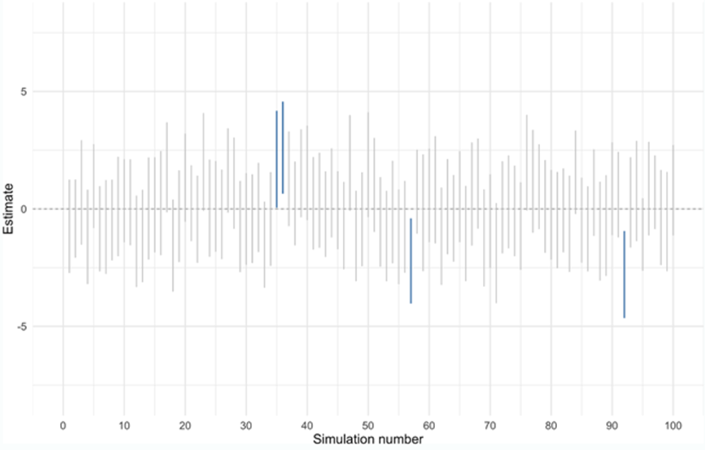
This property of 95% confidence intervals is demonstrated in Figure 5.2,2 which shows the results of a simulation in which random samples were drawn again and again, to see how interval estimates behave. Suppose the true effect size for a treatment is zero and each vertical bar represents the confidence interval resulting from a different random assignment of participants to treatment and control groups. As you can see, most intervals overlap with the true parameter value of zero (on the y axis), but we also expect one out of every 20 estimates (5%) to miss the mark (the bars shown in blue). In practice, we would normally only have one sample and wouldn’t know for sure if ours is one of the unlucky cases in which the confidence interval fails to include the true effect. What we do know is that we’ve followed a process that theoretically gives a correct answer 19 times out of 20.
The 95% confidence level is perhaps most common, but we also frequently encounter confidence levels of 90% and 99%. Whatever confidence level we choose, we are accepting that our procedure will yield a false answer some of the time. With a 95% confidence level we expect a 5% error rate, while a 99% confidence level is associated with an error rate of only 1%. There is always a tradeoff when choosing a confidence level. A more conservative level (e.g., 99%) will yield a wider interval, meaning that we are accepting a wider range of values as possible in order to obtain this higher level of confidence that we will avoid an error.
What procedure is used to construct a confidence interval? We will learn the details in Chapter 8. For now, it is enough to know that there are well-established procedures for constructing confidence intervals in various settings, based on assumptions about the data. Even without knowing these exact procedures, you can hopefully begin to see the usefulness of confidence intervals from the examples in this chapter.
5.2.1 Confidence Intervals for Regression
To examine use of confidence intervals for regression, we will return to the example of predicting university grades based on an admissions exam (Section 3.5). The table is shown again here as Table 5.1.
| Coef. | Std. err. | p-value | |
|---|---|---|---|
| verb_sat | 0.0017 | 0.0010 | 0.10 |
| math_sat | 0.0048 | 0.0012 | 0.00014 |
| (intercept) | -0.91 | 0.42 | 0.033 |
| n | 105 | ||
| r^2 | 0.487 |
Because the coefficients we see in the table are just point estimates, confidence intervals can help us better understand the precision of these estimates by providing us with a range of plausible values for the coefficients. Notice that no confidence intervals have been provided in the table (which is a situation you may frequently encounter when reading social scientific research publications). Fortunately, we can easily calculate a good approximation of a confidence interval for a coefficient estimate \(\hat{\beta_i}\) as long as we also have its standard error estimate (\(s_{\beta_i}\)), which is provided in the table (in the column label “Std. err.”).3 We will learn exactly what a standard error is in Chapter 8, but for now, we can simply insert the standard error estimate into the following formulas:
\[ \text{Lower bound} \approx \hat{\beta_i} - 2\times s_{\beta_i} \]
\[ \text{Upper bound} \approx \hat{\beta_i} + 2\times s_{\beta_i} \]
Note that these formulas are just an approximation for a 95% confidence interval; the formulas for precise intervals are shown in Section 8.3.3. Multiplying the standard error by two yields the approximate margin of error.4 From our initial point estimate of the slope, we can then add or subtract the margin of error to identify a full range of plausible values.
Our approximation approach provides an inexact but close approximation of a 95% confidence interval as long as the sample size is reasonably large (e.g., at least 30 more observations than the number of independent variables included in the regression). In this case, there are 105 observations and only two independent variables, so we will obtain a good approximation. And an approximation is usually the best we can hope for when calculating confidence intervals by hand from a regression table, since we will usually also lose some precision due to rounding error.
For the verbal SAT scores, we find the following bounds:
\[ \text{Lower bound} \approx 0.0017 - (2)(0.0010) = -0.0003 \]
\[ \text{Upper bound} \approx 0.0017 + (2)(0.0010) = 0.0037 \]
This is very close to the precise 95% confidence interval that one finds using statistical software to compute an exact interval: [-0.0003, 0.0038]. Any values within this range can be considered plausible values for the coefficient, according to our model results.
How do we interpret this confidence interval? Remember that when it comes to interpreting size, the coefficient indicates how many units the prediction for the dependent variable changes when the independent variable increases by one unit. But with SAT scores, a 1-unit increase is so small that we found it more useful to consider a 100-point increase, which required multiplying the coefficient by 100. Doing so here, we can conclude that a 100-point increase in the verbal SAT score (e.g., comparing a student with a 600 to a student with a 500, assuming math SAT scores are equal) predicts a difference in the computer science GPA somewhere in the range of [-0.03, 0.38]. Zero is part of this range, so it’s entirely plausible that there is no real association between verbal SAT score and computer science GPA (hence, the lack of statistical significance for this relationship). According to the model results, it is also plausible that a 100-point increase in verbal SAT is associated with the predicted computer science GPA decreasing by as much as 0.03, or increasing by as much as 0.38. A 0.03 decrease in GPA is tiny, so we might feel comfortable ruling out the possibility that a good verbal SAT score has any substantial negative predictive effect for computer science GPA. But a positive effect of 0.38 grade points is much more substantial, so it is plausible that the verbal SAT has a meaningfully-large positive association with computer science GPA.
What about the math SAT? Using our approximation method:
\[ \text{Lower bound} \approx 0.0048 - (2)(0.0012) = 0.0024 \]
\[ \text{Upper bound} \approx 0.0048 + (2)(0.0012) = 0.0072 \]
Multiplying these two values by 100, we find that a 100-point increase in the math SAT is plausibly associated with an increase of between 0.24 and 0.72 points in predicted computer science GPA.
5.2.2 Interpreting Confidence Intervals Correctly
Suppose we want to estimate the average poverty rate for a city based on a sample of residents who have completed a survey. We might calculate a confidence interval and obtain the values [13.4%, 15.1%]. A common mistake made by students and scientists alike when describing this 95% confidence interval is to say “this means there is a 95% chance that the true poverty rate is between 13.4% and 15.1%.” One reason this interpretation is too simplistic is that there may be other relevant evidence about the poverty rate beyond the data used to compute our confidence interval. If several other high-quality studies of the city have recently estimated the poverty rate and produced results in the range of 17-20%, we would probably conclude that our own interval estimate has a good chance of being wrong (much greater than 5%).
So what is the correct interpretation of a confidence interval? You can make the following statement any time you encounter a 95% confidence interval (of the form [A, B]):
Using a process with 95% accuracy (in theory), it is estimated that the parameter lies between A and B.
I realize this interpretation is a bit indirect; it is difficult to provide a technically-accurate and meaningful interpretation, despite the fact that confidence intervals have demonstrated great practical value to researchers and analysts.5 What makes interpretation difficult is the fact that the “% confidence” in a “95% confidence interval” refers to the accuracy of the process of creating a confidence interval—not the probability that a specific confidence interval we encounter will contain the true population parameter. If this distinction seems confusing, it is!
Fortunately, even if you miss the precise details, you will still probably get something useful out of confidence intervals.6 Nonetheless, let’s try to set the record straight.
An analogy may help. Suppose you are interacting with a chatbot that is truthful 95% of the time and lies the other 5%.7 For each statement, will you always conclude it has a 95% chance of being true? Not necessarily. If the chatbot discusses a topic you already know a lot about, you will probably be able to pick out the lies from the true statements with fairly high confidence. Some things the bot says will be things you know to be true, so you can be nearly 100% sure they are true. Other statements will be things you’re quite sure are wrong, so you will conclude that the probability they are true is close to 0%. If you wanted to be very systematic, you could even use the mathematical formula known as Bayes’ theorem8 to combine your prior knowledge of a statement’s probability of being true with the fact that a 95%-accurate bot claimed the statement was true, allowing you to precisely quantify how confident you should be about the statement’s truth in the end.
Now imagine you ask this same bot to start telling you about a topic you know nothing about. Absent any prior insights into which statements are likely to be true, it would now be reasonable to conclude that each statement the bot makes has a 95% chance of being true.
In the same way, it turns out that absent any other information, a 95% confidence interval is often a good approximation for a range of values that contains the population parameter with 95% probability.9 Thus, I think it is quite reasonable that many of us, when we see a mean estimate with a 95% confidence interval ranging from A to B, assume there is a 95% chance the population mean does indeed lie between A and B. But technically, that is not a direct interpretation of the confidence interval; instead, this statement about plausible values of the population mean is a subjective conclusion that I can draw based on the confidence interval. Another person might see the same confidence interval and reasonably decide—drawing on their own prior knowledge of the topic—that the confidence interval contains values that are highly implausible, and thus they would reach a different conclusion from me about how likely the interval is to contain the true population mean.
If you want to elaborate on how the 95% confidence interval [A, B] can inform our practical understanding, you might add the following to our earlier interpretation:
Assuming no additional information and an appropriate statistical model, this result usually suggests that we can be about 95% confident the parameter lies between A and B.
5.3 Exercises
- How is inferential statistics different from the data description we’ve focused on in prior chapters?
- Many medical trials involve tracking patients who are randomly assigned to receive either an experimental medication or a placebo (e.g., a sugar pill). In such trials, what is the treatment group, and what is the control group?
- Suppose I am trying to estimate popular support for the Mayor of London using survey data. My dataset contains responses from 1000 people randomly selected from a list of all registered voters in Greater London. What is my sample? What is my population?
- In practice, why would it be difficult to obtain a truly random sample like the one described in the prior question?
- What letters/symbols do we typically use to represent the mean, variance, and correlation in a sample? What about in a population?
- A regression table shows a coefficient of 2.3 with a standard error of 1.1. Calculate a 95% confidence interval for this coefficient, using the approximation we learned in this chapter.
- Under what condition is the approximation used for the previous question not dependable?
- Suppose I want to know whether I can conclude that an association between two variables is close to zero (meaning they are essentially unrelated). I have estimation results for a regression describing the association of interest. What inference tool from this chapter is most appropriate for helping me discern if the association is near-zero?
Increasing sample size at the expense of other design considerations is not always wise. For example, a very large convenience sample is not necessarily better than a smaller probability sample.↩︎
This image is shared under CC-BY 4.0 and is adapted from Figure 1 of Nalborczyk, L., Bürkner, P. C., & Williams, D. R. (2019). Pragmatism should not be a substitute for statistical literacy, a commentary on Albers, Kiers, and van Ravenzwaaij (2018). Collabra: Psychology, 5(1), 13. https://doi.org/10.1525/collabra.197↩︎
Some publications list t scores or z scores instead of standard errors. These t (or z) scores are typically just the coefficient divided by the standard error estimate, so you can obtain the standard error estimate by dividing the coefficient (\(\hat{\beta_i}\)) by its t score (\(t_{\beta_i}\)): \(s_{\beta_i}=\hat{\beta_i}/t_{\beta_i}\).↩︎
Two is the approximate value by which the standard error should be multiplied, but a more exact value can be found using the t distribution, as explained in Section 8.3.↩︎
Stephens, M. (2023). The Bayesian lens and Bayesian blinkers. Philosophical Transactions of the Royal Society A, 381(2247), 20220144.
Kass, R. E. (2011). Statistical inference: The big picture. Statistical science: a review journal of the Institute of Mathematical Statistics, 26(1), 1.↩︎
Anderson, A. A. (2019). Assessing statistical results: magnitude, precision, and model uncertainty. The American Statistician, 73(sup1), 118-121.↩︎
This example is adapted from Behar, R., Grima, P., & Marco-Almagro, L. (2013). Twenty-five analogies for explaining statistical concepts. The American Statistician, 67(1), 44-48.↩︎
See https://onlinestatbook.com/2/glossary/bayes.html or https://onlinestatbook.com/2/probability/bayes_demo.html.↩︎
Kass, R. E. (2011). Statistical inference: The big picture. Statistical science: a review journal of the Institute of Mathematical Statistics, 26(1), 1.
Albers, C. J., Kiers, H. A., & van Ravenzwaaij, D. (2018). Credible confidence: A pragmatic view on the frequentist vs Bayesian debate. Collabra: Psychology, 4(1), 31.
Greenland, S., & Poole, C. (2013). Living with p values: resurrecting a Bayesian perspective on frequentist statistics. Epidemiology, 24(1), 62-68.↩︎