3 Relationships Between Two Quantitative Variables
When analyzing data, we often want to know how variables are related to one another. For example, we might wonder to what extent a country’s political stability is related to its level of wealth. Supposing we had a dataset containing measures of political stability and wealth, we could use what we learned in the prior chapters to describe the distribution of the political stability measure and of the wealth variable. But we have not yet learned how to assess whether and how two variables are linked. This chapter begins to explore these questions, with a focus on quantitative variables. The next chapter will then extend this discussion to qualitative variables.
3.1 Scatter Plots and Correlation
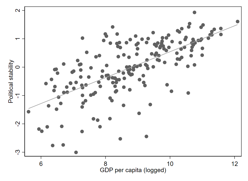
Visually, we can depict the relationship between two quantitative variables using a scatter plot. Figure 3.1 shows an example using data from the 2018 World Bank Development Indicators dataset.1 Two variables are depicted: a common measure of country wealth (logged per capita GDP) and an estimate of perceived political stability that the World Bank generates by combining several data sources. This latter measure is reported in standardized units (z-scores).
Each observation in a scatter plot is shown as one dot, with the x-axis showing values for one variable (GDP per capita in Figure 3.1) and the y-axis representing the other variable (political stability). It is also common to add a straight line, called a regression line, showing the general trend in the data. In this first example, the regression line slopes upward from left to right, so we say there is a positive relationship between the two variables. A positive relationship means that when values of one variable are higher, values of the other variable also tend to be higher. If the line slopes downward, we say there is a negative relationship. With a negative relationship, higher values for one variable correspond to lower values for the other variable.
If we want a single number to summarize the relationship between two variables, we can use a correlation coefficient. A correlation, represented by the letter “r” (\(r\)), always falls between -1 and 1. It tells us two things. First, the sign indicates the direction of the relationship (positive or negative). Second, it tells us how strong the relationship is. Numbers closer to 0 indicate weaker relationships, while numbers closer to 1 or -1 indicate stronger relationships.
For this first example, the correlation is 0.66, which indicates a positive and moderately strong relationship. The correlation matches what we see visually: it is clear that typical values for political stability tend to be higher when GDP per capita is higher. We can therefore say there is a clear, positive association between wealth and political stability (the terms “association” and “relationship” are interchangeable).
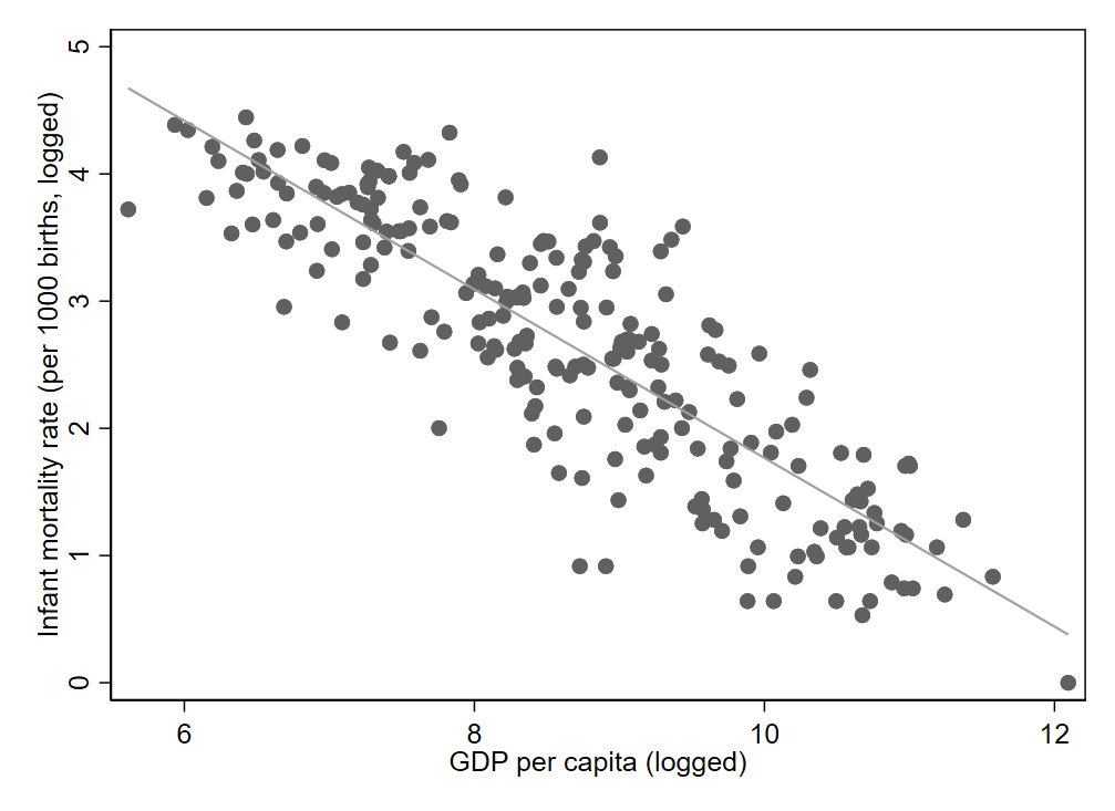
Figure 3.2 shows an example of a negative relationship. The correlation is -0.86. Wealthier countries tend to have lower infant mortality rates. The data in this scatter plot also appear to track more closely to the regression line than in our prior example. Notice that the absolute value of this correlation (0.86) is larger than that of the previous example (0.66), indicating a stronger relationship. Thus, we can say that the wealth-infant morality relationship is stronger than the wealth-political stability relationship.
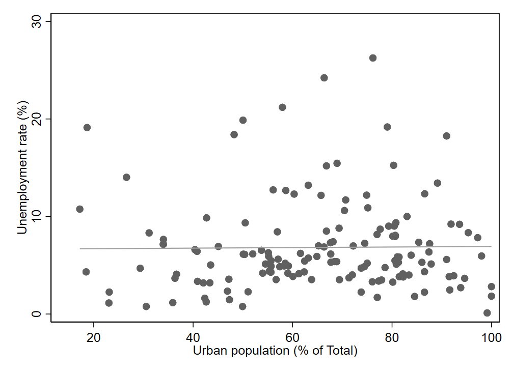
As another example, consider Figure 3.3. The data does not clearly follow any upward or downward trendline. In fact, the regression line in the graph is almost completely flat. The correlation is 0.01, which is very close to 0. Thus, there appears to be no relationship between the variables of urban population and unemployment rate.
Note that a scatter plot can be redrawn by changing which variables are assigned to the x- and y- axes. It is standard practice, however, to choose which variable goes where based on a judgement about the likely cause-and-effect (or predictive) relationship between the two variables. Specifically, we usually depict the variable that we assume is the cause on the x-axis. We call this the independent variable. The y-axis shows the dependent variable, which is the one we believe could be affected (or predicted) by the other variable. In some cases, causal ordering is unclear and we have no intention to predict, so the graph can be drawn either way. Our first scatter plot (Figure 3.1) is an example of an unclear case: wealth might improve stability, but stability might also enable wealth creation.
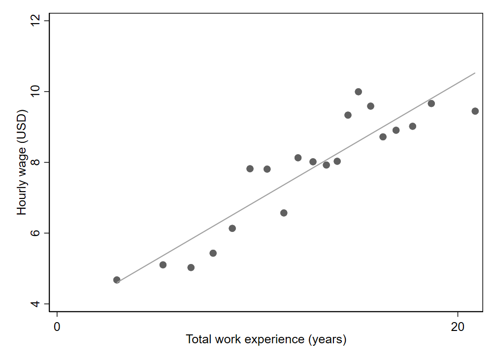
With large datasets, scatter plots can be difficult to interpret since observations tend to stack on top of one another (often leaving only outliers to show up distinctly). The positive association between work experience and wages in Figure 3.4 is not particularly strong, but it is a bit difficult to discern exactly what is going on because the graph is crowded with so many observations (2,246 in total).2 Larger samples will make this problem even worse.
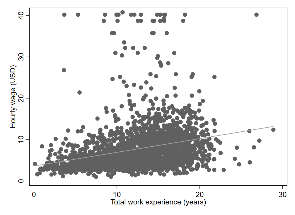
Fortunately, we can create what is called a binned scatter plot. Rather than plotting every observation, we can divide the x axis into bins and plot just one dot per bin. The dot will indicate the mean or median value of the y variable among observations within that bin. While binned scatter plots can bring greater clarity when working with large datasets, be aware that binned scatter plots tend to make relationships look stronger than they really are. This is because aggregating data (by bin, in this case) tends to reduce the noisiness associated with idiosyncrasies in individual observations. See how clear and consistent the relationship between work experience and wages appears in the binned scatter plot (Figure 3.5), despite the relatively weak relationship in the individual-level data (\(r=0.27\)). Notice too that the ranges of both axes have changed, resulting in a regression line that looks much steeper than in the original scatter plot (Figure 3.4). This happened by default in the software used to create the graph, since the binning procedure produced a narrower range of values. By manually adjusting the graph’s settings, the axes could be redrawn to match the original graph.
3.2 Straight Lines and Measuring Correlation
There are multiple types of correlation coefficients, but the one we’ve been using is Pearson’s correlation coefficient. It is the most widely used and the one that is implied when people refer to a “correlation coefficient” without further clarification. Pearson’s correlation coefficient describes the linear relationship between two variables, so it indicates strength of association by telling us how closely the data follow a straight line. A value of 1 or -1 means that the data fall perfectly along a straight line. The closer the absolute value of the Pearson’s correlation is to 1, the better the data track with a straight line. The closer the correlation is to 0, the more the data defy any pattern conducive to us drawing an upward or downward sloping line through them (the data may still appear to follow a perfectly flat line).
Figure 3.6 shows an example of a perfect correlation. Any variable has a correlation of 1 with itself, and here we see that a variable also has a correlation of 1 with a linear transformation of itself (i.e., a standardized version of the variable, something we learned about in the prior chapter). Both axes are depicting the same variable, just expressed in different units (notice the different values on the two axes).
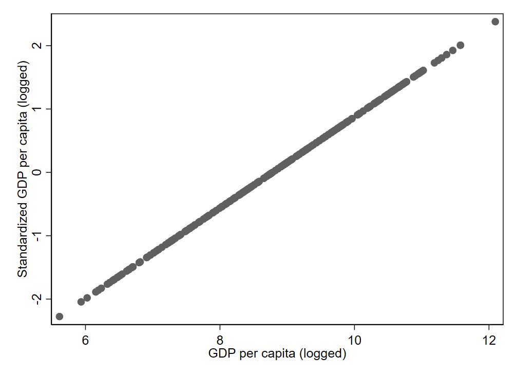
Because Pearson’s correlation measures linear relationships, data that perfectly follow a curved line will not have a correlation of 1. Figure 3.7 shows GDP per capita plotted against its log transformation. Because log transformations are non-linear transformations, the data does not follow a straight line. The correlation of 0.79 indicates that the data still maps reasonably well to the straight regression line shown in the figure, but this coefficient falls well short of 1 even though we can perfectly determine the value of y (logged GDP per capita) if we know the value of x (GDP per capita). Put differently, there is a perfect relationship between the two variables—just not a linear one. Of course, the reason there is a perfect relationship is because one variable is a transformed version of the other variable. We do not normally expect to encounter variables that are perfectly related unless they are measuring they exact same thing.
One implication of relying on a measure of linear association is that a correlation of 0 can mask non-linear relationships. Specifically, a Pearson’s correlation of 0 indicates that there is no linear association between two variables, but it is still possible for a relationship between variables to exist that cannot be approximated meaningfully with a straight line. This is one reason it is usually helpful during analysis to inspect data visually in addition to observing numerical summaries. Doing so may reveal patterns that standard statistics (like Pearson’s correlation) are not well equipped to handle. In Chapter 11, we will learn more about ways to build statistical models for non-linear relationships.
3.3 How Correlation is Calculated
There are many ways to write the formula for correlation. As we saw in the prior chapter, we make a distinction between statistics for a “sample” versus a “population” when writing equations for certain statistics (e.g., variance). It is more common to have data from a sample, but we will focus here on a formula describing the population since it is a bit simpler. Additional formulas (including for samples) are presented in the appendix. Note that we use the Greek letter \(\rho\) (rather than \(r\)) to represent the correlation when we are describing a population.
Here is one way to calculate correlation:
\[ \rho =\frac{1}{N} \sum_{i=1}^{N} \left( \frac{x_i-\mu_x}{\sigma_x} \right) \left( \frac{y_i-\mu_y}{\sigma_y} \right) \tag{3.1}\]
Let’s try to make sense of Equation 3.1 by breaking it up into parts, starting from within the summation.
\(\left( \frac{x_i-\mu_x}{\sigma_x} \right)\) looks like the formula for standardization we learned last chapter, except now we have added some subscripts because we are working in the context of two different variables: \(x\) and \(y\). Adding \(x\) as a subscript to \(\mu\) and \(\sigma\) clarifies that we are referring to the mean and standard deviation of \(x\). With this part of the equation, we are converting the values of \(x\) to z-scores. We can use \(z_x\) to indicate z-scores of \(x\), and we can use \(z_{x_i}\) to indicate that we are describing the z-score of \(x\) for observation \(i\):
\[z_{x_i} = \frac{x_i-\mu_x}{\sigma_x}\]
Similarly, the second set of parentheses in Equation 3.1 indicates that we should generate z-scores for \(y\):
\[z_{y_i} = \frac{y_i-\mu_y}{\sigma_y}\]
Thus, we can re-write Equation 3.1 as:
\[ \rho =\frac{1}{N} \sum_{i=1}^{N} z_{x_i} z_{y_i}=\frac{\sum_{i=1}^{N} z_{x_i} z_{y_i}}{N} \]
This makes it clear that after standardizing our two variables (\(x\) and \(y\)), we multiply them together and then take the average of this product across all observations \(i\) in our dataset to find the correlation.
Table 3.1 shows one way to compute a correlation manually in a spreadsheet. Only 9 observations are shown in the table, but the full dataset consists of 204 observations. The means at the bottom of the table are computed from the full dataset.
In Table 3.1, we see that the variables stability and urban have been transformed to z-scores (columns labeled z_stability and z_urban).3 In the final column, the values of the z-scores for the two variables are multiplied together. The average of this final column shown at the bottom of the table indicates the correlation between stability and urban: 0.36. Thus, there is a weak but noticeable positive association between the two variables.
| id | country | stability | urban | z_stability | z_urban | z_stability × z_urban |
|---|---|---|---|---|---|---|
| 1 | Afghanistan | -2.76 | 25.50 | -2.73 | -1.46 | 3.99 |
| 2 | Albania | 0.37 | 60.32 | 0.40 | 0.00 | 0.00 |
| 3 | Algeria | -0.84 | 72.63 | -0.80 | 0.52 | -0.42 |
| 4 | American Samoa | 1.22 | 87.15 | 1.25 | 1.13 | 1.41 |
| 5 | Andorra | 1.42 | 88.06 | 1.45 | 1.17 | 1.69 |
| 6 | Angola | -0.34 | 65.51 | -0.30 | 0.22 | -0.07 |
| 7 | Antigua and Barbuda | 0.84 | 24.60 | 0.87 | -1.50 | -1.31 |
| 8 | Argentina | 0.01 | 91.87 | 0.04 | 1.33 | 0.06 |
| 9 | Armenia | -0.44 | 63.15 | -0.41 | 0.12 | -0.05 |
| … | … | … | … | … | … | … |
| Mean | -0.03 | 60.26 | 0.00 | 0.00 | 0.36 | |
| N=204 |
This same data is depicted in Figure 3.8, with id numbers used to plot the 9 observations shown in Table 3.1; the remainder of the observations are plotted as circles.
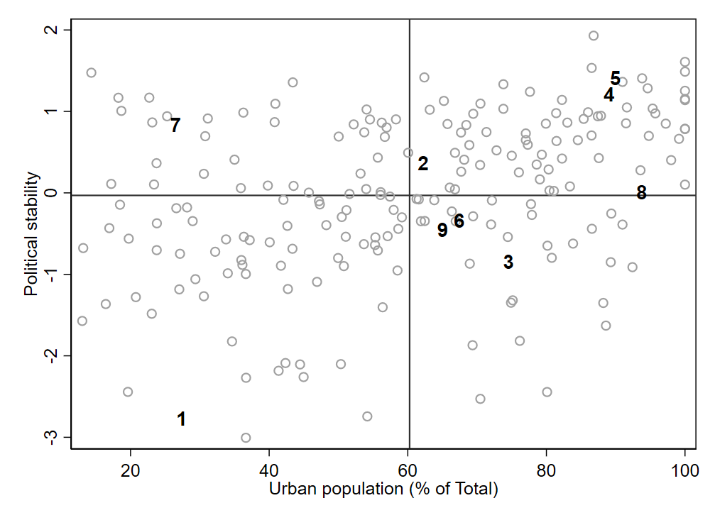
Let’s consider some of the mechanics underlying the calculation of correlation coefficients. By transforming values to z-scores, we indicate where each observation lies relative to the variable’s mean. A positive z-score indicates that the original value of the variable is above the mean while a negative z-score tells us it is below the mean. Visually, we can also see this in Figure 3.8, where a vertical line indicates the mean of urban and a horizontal line marks the mean for stability. This divides the observations into four quadrants. The observations in the upper-right quadrant (including observations 2, 4, 5, and 8) have positive z-scores for both variables. Multiplying two positive values results in a positive value, so all observations in this quadrant also have a positive value in the final column of the spreadsheet previewed in Table 3.1. The bottom-left quadrant contains observations that have both below-average political stability and a below-average urban population (e.g., observation 1). Since this results in two negative z-scores being multiplied together (and the product of two negative numbers is always positive), we again see positive values in the final column of the spreadsheet. The two remaining quadrants will yield negative values in the final column because one z-score will be negative and the other positive (and the product of a negative and a positive number is negative). The upper-left quadrant has below-average values (negative z-scores) for urban but above-average values (positive z-scores) for stability (e.g., observation 7). In the bottom-right quadrant, the share of the population that is urban is above average but stability is below average (e.g., observations 3, 6, and 9).
Since the correlation is the mean of the final column, we can imagine the observations with positive values in the final column “pushing” the correlation toward a positive value while the observations with negative products “push” the correlation toward a negative value. From Figure 3.8, we can see that there are more observations in the two quadrants yielding positive products (upper-right and bottom-left) than in the two “negative” quadrants (upper-left and bottom-right). Thus, it should come as no surprise that the correlation is positive (0.36).
As illustrated in the example above, multiplying two standardized values together results in a positive value any time both variables are above average. This maps neatly to our conceptual definition of a positive relationship: when values of x tend to be higher (above average), values of y also tend to be higher (above average). Thus, finding above-average values for x being paired with above-average values of y (the upper-right quadrant) is consistent with the notion of a positive relationship (as are below-average x values paired with below-average y values, the lower-left quadrant). A negative relationship means that higher values of x (above average) tend to go with lower values for y (below average), so the combination of a positive z-score for x and a negative z-score for y (or vice versa) is consistent with a negative relationship.
3.4 Introduction to Linear Regression
As you have already seen, we often use a regression line to help demonstrate the relationship between two variables when creating a scatter plot. More broadly, regression techniques turn out to be incredibly powerful and are widely used throughout the social sciences. Regression lines are often reported using numbers in tables or equations, so it is important to understand how they can be represented in such formats and not just visually in a graph.
You may recall from geometry that straight lines can be represented with an equation of the following form:
\[ y = mx + b \]
where \(m\) represents the slope and \(b\) represents the y-intercept. By changing the values of \(m\) and \(b\), we can represent any straight line.
In the context of regression, we usually rearrange the terms and change the notation a bit. We can add a hat (^) above \(y\) to indicate that we are making a prediction for the value of \(y\), and we will also add the subscript \(i\) to indicate that the equation is used to make a prediction for each observation in the dataset. We use \(\alpha\) to represent the y-intercept, which we usually just call the intercept, and we use \(\beta\) to indicate the slope coefficient. Finally, we can add the subscript \(i\) to \(x\) just like we did with \(y\):
\[ \hat{y_i} = \alpha + \beta x_i \]
How do we select exactly where to draw the regression line? There are multiple methods, but the most widely used one is called “least squares” because it involves minimizing the squared errors of prediction. “Error of prediction” refers to the difference between the predicted value of \(y\) and the actual value of \(y\) for each observation. There are well-known formulas for selecting \(\alpha\) and \(\beta\) that result in the line that minimizes the sum of the squared errors. These formulas for ordinary least squares (OLS) regression are shown in the appendix.
When we are working with regression, it becomes crucial to distinguish between the independent and dependent variables. \(y\) will always represent the dependent variable, since it is the variable we are trying to predict based on the value of \(x\). Note that calculating a correlation coefficient does not require you to make this distinction: the correlation of \(x\) with \(y\) equals the correlation of \(y\) with \(x\). But when we “run a regression” (meaning we estimate a regression equation), we must specify which variable is the dependent variable. The solution often differs depending on which variable is designated the dependent variable.4
Lane and colleagues5 offer a simple example of regression being used to predict university student performance based on high school (secondary school) performance. Performance is measured using the standard U.S. grade point system, in which students receive letter grades that are scored between 0 and 4 (e.g., A=4, B=3, C=2, D=1, F=0). Students receive separate grades in each class they take, so their overall performance is measured as a grade point average (GPA).
The dataset consists of observations from 105 students who completed a computer science degree at a state university. The two variables being examined in this initial example are the GPA achieved during university studies and GPA during high school.
Using the least squares formulas for estimating a regression line, Lane finds that university GPA can be predicted with the following equation:
\[ \widehat{university\_gpa}_i = 1.097 + 0.675 \times highschool\_gpa_i \]
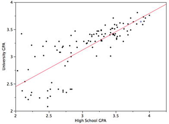
This line is depicted visually in Figure 3.9. The correlation for the two variables is 0.78.
We can plug in any number we want for highschool_gpa to see what the resulting prediction is. For example, we can see what the prediction is for students who had a high school GPA of 2.8:
\[ \widehat{university\_gpa} = 1.097 + 0.675 \times (2.8) \]\[ = 1.097 + 1.89 = 2.987 \]
So a student with a GPA of 2.8 in high school is predicted (based on this sample) to have a slightly higher university GPA of around 3.0 by the time they graduate. This also tracks with what we see in Figure 3.9: if we find 2.8 on the x axis and then draw a straight line up to the regression line, we can see that the height of this point on the regression line appears to correspond to approximately 3.0 on the y axis.
If we stop and think about about the second Question to Always Asks about Data (who is in the dataset?), we might realize the need to add an important caveat to this analysis. The sample only includes university students who completed their degree, but many people who complete high school will never go to university. And even among those who do attend university, those with very poor grades at university are at higher risk of dropping out. Thus, the regression analysis here is unlikely to tell the full story of how high school GPA is related to academic performance at a university, since we don’t get to see from this sample how high school GPA affects the rate of completing a university degree in the first place. We only see the final grade point average among students who do complete their degrees.
3.5 Quick Guide to Interpreting Regression Results
Many social science papers report their main results in the form of a regression table. It’s fairly easy to get started interpreting these results using the three S’s:6
Significance: Is the relationship between the two variables strong enough (relative to the precision of the estimate) to be considered statistically reliable?7 To assess this, check the p-value. For now, you can use the following rule-of-thumb:
If p < 0.05: the relationship is statistically significant; proceed to evaluating sign and size
If p > 0.05: results are somewhat indeterminate; any association detected between the two variables could easily be caused by coincidence or random “noise” (so you may want to skip evaluating sign and size)
Sign: Is the relationship positive or negative? Check whether the coefficient has a negative value.
Positive coefficient: as the independent variable increases, our prediction for the dependent variable increases
Negative coefficient: as the independent variable increases, our prediction for the dependent variable decreases
Note about odds ratios: For certain types of (non-linear) regression, odds ratios (which always take on positive values) are sometimes displayed instead of coefficients; with an odds ratio, a value greater than one indicates a positive relationship while a value smaller than one indicates a negative relationship
Size: How big is the (predictive) effect? This S is often the most difficult to make sense of, and sometimes you may not have enough information to meaningfully evaluate it (e.g., if the units of measurement for a variable are not clearly explained).
For linear models: When the independent variable increases by one unit, we adjust our prediction for the dependent variable by \(\hat{\beta_i}\) (where \(\hat{\beta_i}\) represents the value of the coefficient estimate)8
For non-linear models (e.g., logit, probit): Interpreting the size of a coefficient is typically more complicated than for a linear model; look for the authors’ explanation of effect size or “magnitude” of association
Table 3.2 provides an example of regression results in a format similar to what you may encounter in many research publications. Note, however, that many publications do not list exact p-values; instead, they often use one or more asterisks (*) to denote coefficients with p-values smaller than 0.05 (sometimes also flagging p-values falling below various other thresholds).
| Coef. | Std. err. | p-value | |
|---|---|---|---|
| verb_sat | 0.0017 | 0.0010 | 0.10 |
| math_sat | 0.0048 | 0.0012 | 0.00014 |
| (intercept) | -0.91 | 0.42 | 0.033 |
| n | 105 | ||
| r^2 | 0.487 |
Table 3.2 was created by analyzing the same dataset described in the previous example, although with different variables. The dependent variable is now university GPA in computer science classes. Instead of high school GPA, this regression uses students’ university entrance exam scores on the verbal (verb_sat) and math (math_sat) sections of a test called the SAT. The SAT reports scores on a scale of 200 to 800 for each subject, with 800 representing a perfect score.
Until now, we have looked at simple regression, meaning there is just one independent variable. But in Table 3.2, we find results for a regression where two independent variables (verb_sat and math_sat) are jointly used to predict students’ GPA in computer science classes. It turns out that regression can easily be performed with multiple independent variables, as will be further described in Chapter 11. When we have multiple independent variables, we evaluate each one on its own terms when working through the three S’s. We can interpret the results in Table 3.2 as follows:
verb_sat: The p-value for this variable (0.10) is greater than 0.05, so this variable is not statistically significant. This means we could not establish a reliable link between verbal SAT scores and computer science GPA. Maybe there is no link, or maybe we would need more data to detect the link.9 Since we don’t find statistical significance, we don’t necessarily need to interpret the sign or size.math_sat: The p-value (0.00014) is smaller than 0.05, somath_satis a statistically significant predictor of computer science GPA. The coefficient (0.0048) has a positive sign, so students with higher math SAT scores are predicted to have higher computer science GPAs. When it comes to size, a one-point increase in math SAT (e.g., someone with a 501 versus someone with a 500) yields a prediction for the computer science GPA that is 0.0048 points higher. That seems very small, but a one-point increase on an SAT is barely noticeable (and not actually possible since scores are always multiples of ten). In this case, we can get a better sense of size if we consider an increase of 100 points in the math SAT, which requires multiplying the coefficient by 100. A 100-point increase in the math SAT (e.g., someone with a 600 versus someone with a 500) predicts a computer science GPA that is 0.48 points higher (\(0.0048 \times 100 = 0.48\)). This is nearly half a grade point higher and would be quite noticeable to most students. Thus, the size of predictive effect now seems reasonably large.
Note that we do not need to apply the three S’s to the intercept (which some publications label the “constant”) because it is not a variable. Table 3.2 also contains some additional information frquently shown in regression tables: standard errors (which we will learn more about in Chapter 8), the sample size (n=105), and r-squared (a statistic often used to describe how well the regression model overall explains variation in the dependent variable).
Remember that the three S’s are just a starting point. But they should be enough to help you follow along a little easier when reading the results sections of many research publications. And notice that the third S (size) helps equip us to address the third Question to Always Ask about Data (“how big is the difference?”). If you’ve started working with a statistical software package by now, you can run your own regression models and try using the three S’s to help you understand the results.
3.6 Exercises
If x is negatively correlated with y, that means that larger values of x are associated with _____________ values of y.
If the data follows an upward sloping line (going left to right), what is the sign of the correlation?
Suppose x and y have a correlation of -0.8 while x and z have a correlation of 0.2. Which pair of variables has a stronger relationship?
If data in a scatter plot appear to closely follow the shape of a U, will there be a strong correlation between the two variables?
With a binned scatter plot, will relationships tend to look weaker or stronger than in a traditional scatter plot?
In the table below, is the independent variable (x) statistically significant? What is its sign? Size?
Coefficients Standard Error t Stat P-value Intercept 0.3907111 0.2158171 1.81 0.087 x -0.1092141 0.2002251 -0.55 0.592 Write the equation for the regression results shown for question 6. Using this equation, find the predicted value of the dependent variable when x is -2.
Suppose I am studying two variables (x and y), and I discover that their correlation is -0.7. If I then run a regression with x and y, what can I say ahead of time about the slope coefficient that I will find?
Chapter 3 Appendix: Formulas for Correlation, Covariance, and Regression Coefficients
If we are working with a sample, we can rewrite Equation 3.1 as:
\[ r=\frac{1}{n-1} \sum_{i=1}^{n} \left( \frac{x_i-\bar{x}}{s_x} \right) \left( \frac{y_i-\bar{y}}{s_y} \right) \tag{3.2}\]
The only real difference (besides notation) is that we divide by \(n-1\) rather than \(N\). That is because we use sample standard deviations (\(s_x\) and \(s_y\)) rather than population standard deviations (\(\sigma_x\), \(\sigma_y\)), and sample standard deviations are computed using \(n-1\) in the denominator.
It is also the case, though, that the correlation coefficient equation can be rewritten without using \(N\) or \(n-1\) at all, because these terms cancel out (as we will demonstrate below). Thus, we get equivalent results for the correlation coefficient (unlike with standard deviation or variance) whether we treat our dataset as a population or a sample; we just need to make sure that our formula for the correlation matches whatever formula we have used to calculate the standard deviations (when using a correlation formula that relies on standard deviations).
Before we show how \(n-1\) can be taken out of Equation 3.2, let’s look at an important and related statistic called “covariance.” The sample covariance, written as \(s_{xy}\) or \(Cov(x,y)\), is:
\[ s_{xy}=Cov(x,y)= \frac{ \sum_{i=1}^{n}(x_i-\bar{x})(y_i-\bar{y}) }{n-1} \]
The population variance is similar, except we divide by \(N\) rather than \(n-1\):
\[ \sigma_{xy}=Cov(x,y)= \frac{ \sum_{i=1}^{N}(x_i-\bar{x})(y_i-\bar{y}) }{N} \]
We can rewrite Equation 3.2 to show the relationship between correlation and covariation:
\[ r=\frac{1}{n-1} \sum_{i=1}^{n} \left( \frac{x_i-\bar{x}}{s_x} \right) \left( \frac{y_i-\bar{y}}{s_y} \right) \]\[ =\frac{1}{n-1} \sum_{i=1}^{n} \frac{(x_i-\bar{x})(y_i-\bar{y})}{s_x s_y} \]\[ =\frac{\sum_{i=1}^{n} (x_i-\bar{x})(y_i-\bar{y})}{n-1} \left( \frac{1}{s_x s_y} \right) \]\[ =s_{xy} \left( \frac{1}{s_x s_y} \right) = \frac{s_{xy}}{s_x s_y} = \frac{Cov(x,y)}{\sqrt{Var(x)Var(y)}} \]
Because variances are never negative values, the denominator of this equation will always be positive (assuming it is not zero). Thus, correlation and covariance will always have the same sign. They both measure association, but covariance is harder to intepret because unlike correlation, covariance is not bounded by -1 and 1. We can have a covariance of -2,000 or 1,000,000. Correlation cannot have an absolute value greater than 1 because the covariance is scaled by the variance of the underlying variables.
Note too that \(Cov(x,x)=Var(x)\). Knowing this, we can demonstrate that any variable has a correlation of 1 with itself:
\[ r_{x,x}=\frac{Cov(x,x)}{\sqrt{Var(x)Var(x)}}=\frac{Var(x)}{Var(x)}=1 \]
Now that we know how to write correlation as a function of covariance and variance (or standard deviation), it is not too difficult to show how to remove \(n-1\) from the equation. We will need to use the formula for the standard deviation from last chapter (\(s=\sqrt{\frac{\sum_{i=1}^{n}(x_i-\bar{x})^2}{n-1}}\)):
\[ r=\frac{s_{xy}}{s_x s_y} = \frac{\frac{\sum_{i=1}^{n}(x_i-\bar{x})(y_i-\bar{y}) }{n-1}}{ \sqrt{\frac{\sum_{i=1}^{n}(x_i-\bar{x})^2}{n-1}} \sqrt{\frac{\sum_{i=1}^{n}(y_i-\bar{y})^2}{n-1}} } \] \[ = \frac{\frac{\sum_{i=1}^{n}(x_i-\bar{x})(y_i-\bar{y}) }{n-1}}{ \frac{\sqrt{\sum_{i=1}^{n}(x_i-\bar{x})^2 \sum_{i=1}^{n}(y_i-\bar{y})^2 }}{n-1} } \] \[ = \frac{\sum_{i=1}^{n}(x_i-\bar{x})(y_i-\bar{y}) }{ \sqrt{\sum_{i=1}^{n}(x_i-\bar{x})^2 \sum_{i=1}^{n}(y_i-\bar{y})^2 } } \]
This final expression is another common way to write the equation for the correlation coefficient. It also helps explain why there is no need to create separate functions (in statistical software) for calculating sample versus population correlations, since there is no need to divide by \(N\) or \(n-1\) or to rely on calculations of variance/standard deviation (which differ for the population and sample).
To conclude this appendix, let’s go over the formulas for OLS estimates of a simple regression line. The formula for estimating the slope is:
\[ \hat{\beta} = \frac{s_{xy}}{s_x^2} = \frac{\sum_{i=1}^{n}(x_i-\bar{x})(y_i-\bar{y}) }{ \sum_{i=1}^{n}(x_i-\bar{x})^2 } \]
As we discussed with correlation, a denominator made up of variances will never be negative. Therefore, the sign of the slope will always be equal to the sign of the covariance (\(s_{xy}\)) and also of correlation (since covariance and correlation always share the same sign).
The estimate of the intercept is:
\[ \hat{\alpha} = \bar{y} - \hat{\beta} \bar{x} \]
US National Longitudinal Survey of Young Women (NLSW), 1988 extract. Accessed via Stata.↩︎
Note that standardizing was accomplished using the population variance formula, in order to match the calculation of the mean for the final column, which divides by N rather than n - 1.↩︎
The main exception is that if we have two standardized variables, the regression slope will be equal to the correlation and the intercept will be 0, so coefficients will be equivalent regardless of which variable is designated the dependent variable.↩︎
David M. Lane. “Introduction to Linear Regression.” Online Statistics Education: A Multimedia Course of Study. https://onlinestatbook.com/2/regression/intro.html↩︎
Wheelan, C. (2010.) Introduction to Public Policy. New York: W. W. Norton & Company.↩︎
In other words, can we conclude it is signal rather than noise? See: Fricker Jr, R. D., Burke, K., Han, X., & Woodall, W. H. (2019). Assessing the statistical analyses used in basic and applied social psychology after their p-value ban. The American Statistician, 73(sup1), 374-384.↩︎
Why \(\hat{\beta_i}\) and not simply \(\beta_i\)? We use the hat symbol (\(\hat{~}\)) to indicate an estimate or prediction. So by including the hat, we are implying that our coefficient is an estimate. We’ll learn more about estimation in Chapter 5.↩︎
The absence of evidence is not necessarily evidence of absence. There could very well be a link between verbal SAT scores and computer science GPA that we cannot reliably detect with this analysis (e.g., because our sample is too small to precisely estimate the association). Confidence intervals (introduced in Chapter 5) will help us evaluate this possibility.↩︎