6 Hypothesis Testing
Hypothesis tests allow us to determine whether a finding is “statistically significant,” an idea we briefly encountered in Chapter 3 when discussing how to interpret regression results tables. Testing for statistical significance is the dominant way that the probabilistic conclusions from inferential statistics are communicated in science. However, many statisticians (and other methodologists) have criticized this broad reliance on significance testing as overly simplistic, confusing, or otherwise ill-founded. Hypothesis testing is important to learn because of its widespread use, but confidence intervals are often more informative for describing statistical results.
As we will see in this chapter, hypothesis testing can often be understood as a particular application of confidence intervals. The risk with hypothesis tests is that we reduce our results down to a binary (significant or not significant), ignoring other nuances that may be present in the results. We will discuss some of these limitations in more detail throughout this chapter.
6.1 Getting Started: A Binary-Quantitative Relationship
We learned in Chapter 4 that we can use a comparison of means to evaluate how a binary (qualitative) variable relates to a quantitative variable. To see how hypothesis testing applies when comparing two means, we will use data describing U.S. congressional districts. Each district elects a single member (a congressperson) to the U.S. House of Representatives. There is a binary variable rural indicating whether a majority of the district’s residents live in a rural area. A quantitative variable ideology is an estimate of the political ideology of the elected official representing that district.1 Ideology can be measured on a continuous left-to-right scale (also called “liberal” to “conservative” in the US political system), with higher values indicating an official is further to the right.
6.1.1 Null and Alternative Hypotheses
The starting point for hypothesis testing is a null hypothesis, which is sometimes just called “the null.” Practically speaking, the null hypothesis usually indicates that there is no relationship between variables.2 So if we are comparing two means, the null hypothesis would typically be that the two means are the same. The null hypothesis always describes a parameter being estimated, not a sample statistic. Therefore, when writing a null hypothesis as an equation, we generally use Greek letters. For example, a null hypothesis may contain one or more instances of \(\mu\), representing a population mean. If there is no clearly-defined population, \(\mu\) might represent the “expected value” (defined in the following chapter) for a variable that we assume was generated through a (partially) random process. This latter interpretation is probably more appropriate to the example data we’re using. \(H_0\) is how we formally denote the null hypothesis, so for our data example we can write:
\[
H_0: \mu_R = \mu_U
\tag{6.1}\] using the subscripts \(R\) and \(U\) to indicate “rural” and “urban,” and \(\mu\) for the expected value (or population mean) of the quantitative variable: ideology. Simply put, this null hypothesis states that the expected value of ideology among rural districts is the same as the expected value of ideology among urban districts.
Another way to write this null hypothesis is:
\[ H_0: \mu_R - \mu_U = 0 \tag{6.2}\]
This indicates that the difference in the expected value of ideology between rural versus urban districts is zero (there is no difference).
As we learned in Chapter 4, we can use a regression equation to indicate a difference in means. Thus, we often rewrite \(\mu_R - \mu_U\) as \(\beta\):
\[ H_0: \beta = 0 \tag{6.3}\]
Note that when analyzing an experimental study, a null hypothesis of this form might be used but with \(\beta\) defined as the average treatment effect.
Every null hypothesis should be paired with an alternative hypothesis, which is the logical opposite of the null hypothesis. We write \(H_A\) (or \(H_1\)) to represent the alternative hypothesis, and our alternative to Equation 6.1 is:
\[ H_A: \mu_R \neq \mu_U \tag{6.4}\]
Or equivalently:
\[ H_A: \mu_R - \mu_U \neq 0 \tag{6.5}\]
Or:
\[ H_A: \beta \neq 0 \tag{6.6}\]
Moving forward, we will focus on the final form in which we’ve written the null and alternative hypotheses (Equation 6.3 and Equation 6.6). We have already learned that confidence intervals can be constructed for regression coefficients, so let’s see if we can evaluate these hypotheses using a confidence interval from a regression.
6.1.2 Evaluating Hypotheses with a Confidence Interval
Table 6.2 presents results for a regression where ideology is the dependent variable and the binary variable rural is the independent variable. The table includes confidence intervals for the coefficients:
| Coef. | Std. Err. | p-value | 95% Conf. Interval | |
|---|---|---|---|---|
| rural | 2.294 | 0.446 | 0.000 | [1.418, 3.170] |
| (intercept) | -0.024 | 0.140 | 0.864 | [-0.299, 0.251] |
| n | 435 | |||
| r^2 | 0.058 |
The row labeled rural corresponds to what we have written as \(\beta\) in our hypotheses. The null hypothesis indicates that \(\beta\) is 0, but the value of 0 is not included within the range identified by the 95% confidence interval (0 is not between 1.418 and 3.170). Thus, we can reject the null hypothesis. The alternative hypothesis indicates that \(\beta\) is not zero, and the 95% confidence interval suggests that \(\beta\) is indeed not zero. Thus, we accept the alternative hypothesis. Given that null and alternative hypotheses are logical opposites, we accept the alternative hypothesis whenever we reject the null hypothesis.
Because we reject the null hypothesis of no relationship between the two variables, we can say that the relationship is statistically significant. We previously learned to draw this same conclusion by noting that the coefficient’s p-value is less than 0.05. It is no coincidence that Table 6.2 indicates a p-value smaller than 0.05 for the rural coefficient, aligning with what we concluded using the confidence interval. The calculation of the p-value follows a process that perfectly aligns with the confidence interval, such that the p-value will always be less than 0.05 when the confidence interval indicates we reject the null hypothesis. It does not matter, therefore, whether we use a confidence interval or a p-value to test a hypothesis. Note that in any regression table, the p-value shown for each coefficient will typically correspond to the null hypothesis stating that the coefficient is 0.
If the 95% confidence interval for the rural coefficient had included 0 (i.e., if the lower bound was negative and the upper bound was positive), we would have failed to reject the null hypothesis.
6.1.3 Substantive Significance
A word of caution about our conclusion here: statistical significance doesn’t mean that the relationship between variables is strong—only that we could reject the possibility of a relationship being entirely absent (i.e., we reject the notion that the expected value of ideology is exactly the same in rural and urban districts). To assess whether a relationship is strong or substantively significant, we need to use tools other than standard hypothesis tests (such as scrutinizing the range of the confidence interval, as we did in the prior chapter). This is one reason I encourage you to always consider “How big are the differences?” (the third Question to Always Ask about Data): many publications clearly indicate statistical significance but do not devote sufficient attention to substantive significance.
In this case, assessing substantive size is a bit difficult because ideology is measured in unfamiliar units. Ideology scores (among congresspersons in this sample) range from -4.10 to 4.57, and the standard deviation is 2.85. Since the smallest number (in absolute value) within the confidence interval for the rural coefficient is its lower bound of 1.42, we can say that the systematic difference between urban and rural districts appears to be at least half a standard deviation (\(1.42 \div 2.85 = 0.498\)). A difference of half a standard deviation is generally considered to be quite large, so we can say that congresspersons from rural districts are notably further to the right politically (more conservative) than congresspersons from urban districts.
While I will not walk through an analysis of substantive size for every example presented in this chapter (for sake of brevity), it is almost always important in applied research to consider substantive strength of associations when interpreting statistically significant findings.
6.2 Testing Relationships for Various Types of Variables
Let’s now consider each possible pairing of qualitative and quantitative variable types and see how a hypothesis test can be applied to each relationship.
6.2.1 Qualitative-Quantitative Relationships
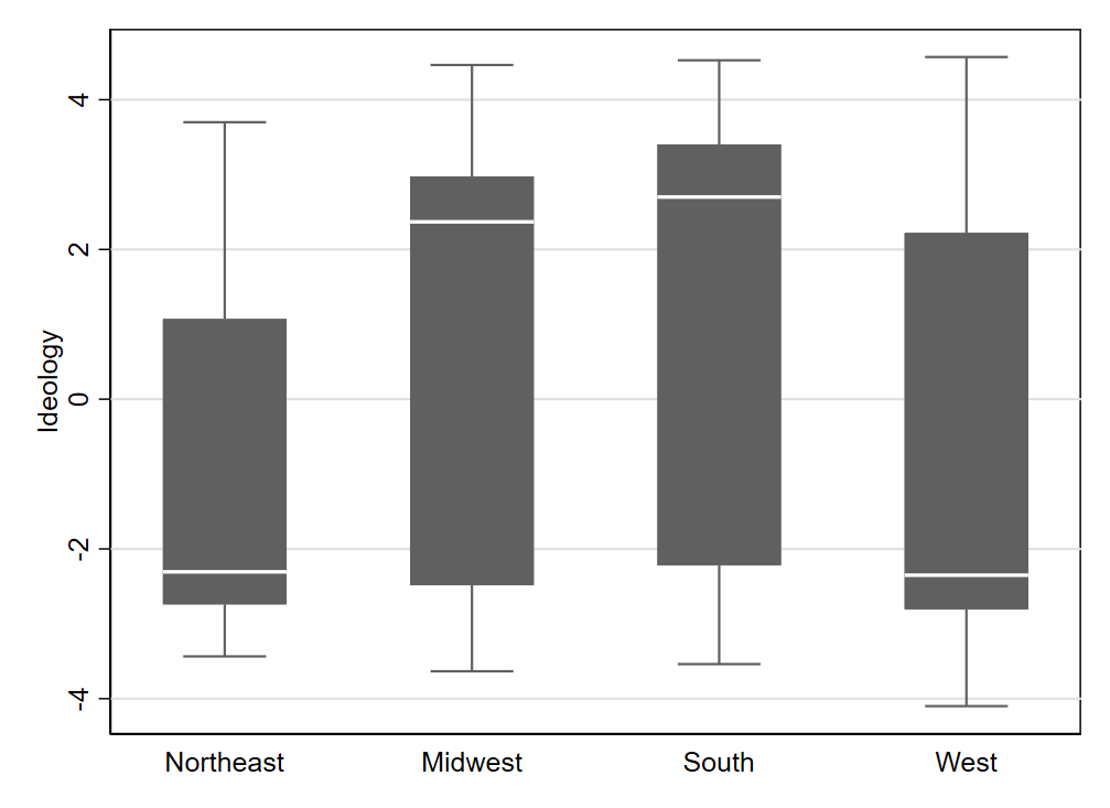
We already saw how to evaluate this when the qualitative variable is binary, but what about when it is not? Table 6.2 shows results for a regression where the independent variable is now the qualitative variable region, coded according to the U.S. Census Bureau’s delineation of the country into four regions.3 Northeast is the omitted category (see Section 4.2.2.2).
| Coef. | Std. Err. | p-value | 95% Conf. Interval | |
|---|---|---|---|---|
| Northeast | - | - | - | - |
| Midwest | 1.885 | 0.413 | 0.000 | [1.074, 2.697] |
| South | 2.602 | 0.369 | 0.000 | [1.878, 3.327] |
| West | 0.468 | 0.401 | 0.244 | [-0.320, 1.256] |
| (intercept) | -1.285 | 0.305 | 0.000 | [-1.884, -0.686] |
| N | 435 | |||
| r2 | 0.140 | |||
| F(3, 431) | 23.35 (p=0.000) |
In this regression, each slope coefficient estimate indicates the difference in means between the given region and the omitted category (Northeast). The null hypothesis should indicate that there is no relationship between the two variables region and ideology, but what does that look like in practice?
6.2.1.1 Null and Alternative Hypotheses
If there is no relationship in this context, then changing the value of region should result in no change in the prediction for ideology. This implies that each pair of differences should be equal to 0, so all regression slope coefficients should be 0 (according to the null hypothesis). We can write this as a single hypothesis, using \(\beta_1\) to indicate the first slope coefficient, \(\beta_2\) to indicate the second slope coefficient, and so on:
\[ H_0: \beta_1 = \beta_2 = \beta_3 = 0 \tag{6.7}\]
If all differences between categories are 0, this implies that the means (or expected values) for all regions are equal, so another way to write this hypothesis is:
\[ H_0: \mu_N = \mu_M = \mu_S = \mu_W \tag{6.8}\] where the subscripts (\(N\), \(M\), \(S\), and \(W\)) indicate each region by its first letter.
What does our alternative hypothesis look like? For the null hypothesis to be false, at least one pair of regions must differ in their population means (or expected values). We can write this formally in either of the following forms:
\[ H_A: \beta_i \ne 0 \text{ for some } i \tag{6.9}\]
\[ H_A: \mu_i \ne \mu_j \text{ for some } i,j \tag{6.10}\]
6.2.1.2 Evaluating Hypotheses with an F Test
How can we use the regression output to evaluate these hypotheses? A natural place to start is by again evaluating the confidence intervals on each slope coefficient: while the coefficient for West could very well be 0 (0 is within the confidence interval), the confidence intervals for Midwest and South both contain all positive (non-zero) values. Thus, we can conclude that the expected value of ideology for congresspersons in the Midwest is different than in the Northeast, and there is also a difference for the South versus the Northeast. This would seem to imply that the null hypothesis (Equation 6.7) should be rejected.
However, this approach of evaluating each slope coefficient one-by-one is not the ideal way to test the null hypothesis indicated in Equation 6.7. Instead, it is better to take an all-in-one approach to match the nature of the hypothesis, which makes a joint statement about three coefficients. While there is no easy way to do this with confidence intervals, we can utilize something called an F test, which provides a p-value like we used initially when learning about statistical significance for regression (in Chapter 3). The typical F test that is performed by default with a regression in statistical software packages tests the null hypothesis that all coefficient slopes are equal to zero, which is exactly what we want in this case. You may have noticed that the bottom of Table 6.2 includes an extra row (not seen in prior regression tables) displaying an F statistic (23.35) and a corresponding p-value (0.000). The exact details of how this F test is conducted are beyond the scope of this book, but you can use what you’ve already learned (in the context of regression slopes) about comparing p-values to a 0.05 threshold to evaluate this null hypothesis. Because this p-value is less than 0.05, we reject the null hypothesis and conclude that at least one slope coefficient is non-zero. Thus, we conclude that regarding congresspersons’ ideology, at least one region has a different expected value (population mean) from another region.
6.2.1.3 Pairwise Comparisons
Note that the alternative hypothesis we accepted in the prior section is particularly vague: we only know that at least one region differs from at least one other region. While this is a meaningful statement in the sense that it tells us region is related ideology, it is a rather open-ended conclusion. Because analysts often want to provide more specific description of differences across categories, it is common when examining a qualitative-quantitative relationship to also evaluate “pairwise” hypotheses that compare only two categories at a time. When there are four categories for the qualitative variable, there are a total of six unique pairings. One way to write the null hypotheses for these six comparisons is as follows:
\[ H_0: \mu_N = \mu_M \]\[ H_0: \mu_N = \mu_S \]\[ H_0: \mu_N = \mu_W \]\[ H_0: \mu_M = \mu_S \]\[ H_0: \mu_M = \mu_W \]\[ H_0: \mu_S = \mu_W \tag{6.11}\]
Table 6.2 allows us to easily test the first three of these pairwise null hypotheses. In fact, we already observed that the first and second hypotheses can be rejected but the third cannot (since the coefficient for West could plausibly be 0, given the 95% confidence interval). It may seem odd that I am returning to evaluating each comparison one-by-one, after I said in the prior section that doing so was not a good way to evaluate Equation 6.7. What is important to highlight is that the way we test the single hypothesis Equation 6.7 is different from how we test a series of pairwise null hypotheses (Equation 6.11). While the distinction can be confusing, since the series of pairwise nulls implies in combination the single combined null, the details of how we evaluate a single hypothesis differ from testing a series of hypotheses. For this reason, it is also possible (though not particularly common) that results for the pairwise hypotheses will appear to contradict results for the single combined hypothesis. Applied researchers commonly use both the combined single hypothesis and the pairwise series of hypotheses, sometimes in combination and sometimes separately. Thus, it is important to be familiar with both approaches to testing a qualitative-quantitative relationship. When results seem to differ from the two approaches, it is hard to give broad advice about which testing approach to favor since researchers apply varied standards, and different research settings may merit different priorities.
Returning to the present example, we said the first three of the pairwise null hypotheses (in Equation 6.11) can be evaluated with the results from Table 6.2, but what about the other three? We can re-specify the regression by changing the omitted category, in order to make the remaining three comparisons. Table 6.3 shows the results, with information corresponding to each coefficient (standard errors, p-values, and confidence intervals) now shown in vertical rather than horizontal format, in order to make space to display four regression models in one table.
| Model 1 | Model 2 | Model 3 | Model 4 | |
|---|---|---|---|---|
| Northeast | - | -1.885 | -2.602 | -0.468 |
| - | (0.413) | (0.369) | (0.401) | |
| - | p=0.000 | p=0.000 | p=0.244 | |
| - | [-2.697,-1.074] | [-3.327,-1.878] | [-1.256,0.320] | |
| Midwest | 1.885 | - | -0.717 | 1.418 |
| (0.413) | - | (0.347) | (0.381) | |
| p=0.000 | - | p=0.040 | p=0.000 | |
| [1.074,2.697] | - | [-1.399,-0.034] | [0.668,2.167] | |
| South | 2.602 | 0.717 | - | 2.135 |
| (0.369) | (0.347) | - | (0.333) | |
| p=0.000 | p=0.040 | - | p=0.000 | |
| [1.878,3.327] | [0.034,1.399] | - | [1.480,2.789] | |
| West | 0.468 | -1.418 | -2.135 | - |
| (0.401) | (0.381) | (0.333) | - | |
| p=0.244 | p=0.000 | p=0.000 | - | |
| [-0.320,1.256] | [-2.167,-0.668] | [-2.789,-1.480] | - | |
| (intercept) | -1.285 | 0.601 | 1.318 | -0.817 |
| (0.305) | (0.279) | (0.207) | (0.261) | |
| p=0.000 | p=0.032 | p=0.000 | p=0.002 | |
| [-1.884,-0.686] | [0.053,1.148] | [0.910,1.725] | [-1.329,-0.305] | |
| N | 435 | 435 | 435 | 435 |
| r2 | 0.140 | 0.140 | 0.140 | 0.140 |
| F(3, 431) | 23.35 (p=0.000) | 23.35 (p=0.000) | 23.35 (p=0.000) | 23.35 (p=0.000) |
Model 1 duplicates (in the new format) what we already saw in Table 6.2. Looking to Model 2, we see that the first coefficient (Northeast) indicates a comparison we already considered in Model 1: the comparison of the Northeast with the Midwest (the new omitted category). The sign of the coefficient has flipped from what it was before (because we have changed which mean we subtract from the other), but otherwise information is identical to what we saw for the Midwest coefficient in Model 1. Across the models, all of the coefficients appearing above the omitted category will turn out to duplicate a comparison we already saw in a prior model, so we will skip over examining these coefficients. Model 4 turns out to be entirely unnecessary, since it only duplicates comparisons that have already been made.
The South coefficient in Model 2 indicates the difference between the South and the Midwest (the omitted category in this model). The confidence interval indicates a range of all-positive (non-zero) values, so we can reject the null hypothesis of no difference between the South and the Midwest. The West coefficient has a confidence interval that contains all-negative values, so we also reject the null hypothesis for the West-Midwest comparison.
In Model 3, we find the final comparison in the West coefficient, which has a confidence interval consisting of all-negative values. Therefore, we reject the null hypothesis of no difference between the West and the South.
Keeping track of this many comparisons can get a bit overwhelming (and will be even more so when a qualitative variable has more than four categories). It is often helpful to create a visualization of the relationship, as we learned in Chapter 4, which we can reference as we evaluate each hypothesis. Figure 6.1 helps make clear why we couldn’t reject a null hypothesis of no difference when it came to the Northeast versus the West: their medians appear to be virtually identical. Note, however, that the ability to find statistical significance also depends on sample size. Two distributions that look very different in a box plot may fail to have a statistically significant difference if the sample size of one or both distributions is very small. In this case, we have a reasonable number of observations (at least 76) in each of the four regions.
The first appendix to this chapter discusses a concern that is often raised when doing a series of (pairwise) hypothesis tests in the manner we have just done. Because we relied on a standard 95% confidence threshold for each estimate we evaluated, our process will generally yield errors more than 5% of the time for at least one estimate we are evaluating (even if all assumptions are met). Exactly what should be done about this is a matter of some debate, and there are multiple ways that researchers conduct pairwise comparisons of means in practice; see the appendix for additional details.
6.2.2 Relationships between Quantitative Variables
If we have two quantitative variables, it is straightforward to test for the statistical significance of the relationship between the two variables. Let us consider the relationship between the geographic size of a congressional district (measured in logged square miles) and the elected member’s ideology.
6.2.2.1 Null and Alternative Hypotheses
A null hypothesis of no relationship between two quantitative variables can be written either using \(\beta\) to represent a regression coefficient or \(\rho\) to represent a population correlation:
\[ H_0: \beta = 0 \tag{6.12}\]
\[ H_0: \rho = 0 \tag{6.13}\]
The alternative hypothesis will be the logical opposite:
\[ H_A: \beta \ne 0 \tag{6.14}\]
\[ H_A: \rho \ne 0 \tag{6.15}\]
Though a simple regression slope coefficient and correlation coefficient normally have different values, their signs are always the same, as noted in Chapter 3. Tests of the above null hypotheses (Equation 6.12 and Equation 6.13) also yield equivalent p-values, so we will obtain equivalent results regardless of which statistic (\(\hat{\beta}\) or \(\hat{\rho}\)) we use for our hypothesis testing. We will focus here on using regression.
6.2.2.2 Evaluating Hypotheses with a Confidence Interval
In Table 6.4, we see a confidence interval for the geographic size coefficient, labeled log_area. The confidence interval ranges from 0.811 to 1.046 and does not include 0. Therefore, we reject the null hypothesis of a regression slope of 0 (meaning we also reject that the correlation could be 0). Note that the p-value is also less than 0.05, which is another way to arrive at the conclusion that we reject the null hypothesis and accept the alternative.
| Coef. | Std. Err. | p-value | 95% Conf. Interval | |
|---|---|---|---|---|
| log_area | 0.929 | 0.060 | 0.000 | [0.811,1.046] |
| (intercept) | -6.687 | 0.456 | 0.000 | [-7.583,-5.791] |
| N | 429 | |||
| r2 | 0.362 |
6.2.3 Relationships between Qualitative Variables
It is not very straightforward to use regression to test whether a relationship between two qualitative variables is statistically significant, so we will use a different approach that builds on the contingency tables we learned about in Chapter 4. To add a test of statistical significance to a contingency table, we can use a test called a Chi Square test. More details can be found in the second appendix to this chapter, but we will focus here on using the p-value resulting from the test to draw a conclusion. Note, however, that the Chi Square test does not work well with very small samples.4
To demonstrate the Chi Square test, we again look to data from the Mediterranean Diet and Health case study,5 in which heart attack survivors were randomly assigned to follow one of two diets. We already discussed in Chapter 4 how the frequencies in Table 6.5 indicate that people on the Mediterranean diet tended to have better outcomes, but we did not say anything previously about the statistical significance of this relationship.
| Outcome | Total | ||||
|---|---|---|---|---|---|
| Diet | Cancers | Fatal Heart Disease | Non-Fatal Heart Disease | Healthy | |
| AHA | 15 | 24 | 25 | 239 | 303 |
| Mediterranean | 7 | 14 | 8 | 273 | 302 |
| Total | 22 | 38 | 33 | 512 | 605 |
As with all other hypothesis tests in this chapter, the null hypothesis indicates no relationship between the two variables. Writing out an exact equation representing the null and alternative hypotheses is not very straightforward, so we will simply use words to describe the hypotheses in this case. The alternative hypothesis indicates that knowing the value of one variable helps us predict the value of the other variable (in the population or in expectation). When conducting a Chi Square test with statistical software, it is common that the software will report both a Chi Square test statistic and a p-value. In this case, the test statistic is 16.55 and the p-value is 0.0009. Because the p-value is less than 0.05, we reject the null hypothesis that the two qualitative variables (diet and health outcome) are unrelated (in the population or in the random process that generated the sample). The relationship is statistically significant.
6.3 Probability Values
While confidence intervals can be used to conduct many hypothesis tests, it is still important to learn about probability values, usually referred to as p-values or just “p.” The basic logic underlying p-values is that we want to consider whether our data would be unusual to observe if the null hypothesis were true. It can be helpful to describe the null hypothesis in terms of indicating a “hypothesized value” for the parameter of interest. We calculate a p-value under the assumption that the parameter is equal to the hypothesized value. The p-value answers the question “If the null hypothesis is true, how likely are we to get a sample statistic as far away from the hypothesized value as the one we got in our sample?” For example, if the null hypothesis states that a regression coefficient \(\beta\) is 0, the p-value is the probability of obtaining a coefficient estimate (\(\hat{\beta}\)) at least as far from 0 as the one we obtained with our sample. The p-value will very much depend on the sample size, since getting estimates that are far from the truth is quite common with small samples. But with a large sample, it would be quite surprising to find a coefficient estimate with a very large absolute value if the true coefficient value was 0.
To help us evaluate p-values, we typically rely on a significance level, referred to as alpha (\(\alpha\)). The alpha level establishes a threshold for deciding at what point a statistical result is “unlikely” enough (under the assumption of a true null hypothesis) that the null hypothesis is rejected. The most common alpha is 0.05, the benchmark we have been referencing so far whenever we have discussed p-values. Any time the p-value is smaller than alpha, we reject the null hypothesis (and accept the alternative hypothesis). Any time the p-value is greater than alpha, we fail to reject the null hypothesis. “Failing to reject” is perhaps clunky language, but it is meant to imply an inconclusive result.
While 0.05 is the standard default alpha, social science researchers also frequently utilize alpha levels of 0.10, 0.01, and 0.001. In many publications, several alphas are used simultaneously. For example, a table may use a plus sign (+) to indicate significance at the 0.10 alpha level, a single asterisk for significance at 0.05 (*), and two asterisks for significance at 0.01 (**). This usage implies that we can evaluate null hypotheses as being rejected with varying levels of confidence: a p-value that is very small (e.g., 0.0004) suggests greater certainty that the null hypothesis is wrong than a p-value that is larger (e.g., 0.08), all else equal.
You may have noticed that significance levels appear to be the flip side of confidence levels. A confidence level of 95% (0.95 as a proportion) implies a significance level of 5% (0.05). That is why we can use a 95% confidence interval to test a null hypothesis with a 0.05 alpha. More generally, the confidence level and corresponding significance level will always add up to 100% (or a proportion of 1). Thus, a 99% confidence interval can be used to test a null hypothesis with an alpha of 0.01, for example.
6.4 Type I and Type II Errors
When discussing the tradeoffs associating with using different alpha levels, we often reference “type I” and “type II” errors. A type I error refers to rejecting a null hypothesis that is actually true. Type I errors are also called “false positives”. A type II error occurs when we fail to reject a null hypothesis that is false.
With a relatively large alpha (e.g., \(\alpha = 0.10\)), we accept a fairly high risk of a type I error. If the null hypothesis happens to be true, we will still reject it at a rate of alpha (10% of the time if \(\alpha = 0.10\)). Setting a lower alpha means that we lower the risk of type I errors, but we increase the risk of type II errors. For example, with an alpha of 0.001, we expect that even if the null hypothesis is true, we will fail to reject it more often because we have set a high threshold for rejecting the null hypothesis.
6.5 One-Tailed and Two-Tailed Tests
So far, our coverage of hypothesis testing has assumed that we are using what is called a two-tailed test. It is also possible to conduct a one-tailed test. A one-tailed test has an alternative hypothesis with a greater-than (>) or less-than (<) sign rather than an unequal sign (\(\ne\)). Returning to the example at the start of this chapter, we could indicate that we are testing whether rural districts have more right-leaning (conservative) congresspersons with this alternative hypothesis:
\[ H_A: \beta > 0 \tag{6.16}\]
Another way to write this would be:
\[ H_A: \mu_R > \mu_U \tag{6.17}\]
There are differing conventions (described in the next section) for how to write a 1-sided null hypothesis, but the clearest approach for our purposes is as follows:
\[ H_0: \beta \leq 0 \tag{6.18}\]
Or equivalently:
\[ H_0: \mu_R \leq \mu_U \tag{6.19}\]
A confidence interval can be used to conduct a 1-tailed hypothesis test, but an adjustment needs to be made for the fact that a 2-tailed confidence interval is being used to conduct a 1-tailed test. Specifically, one should use an interval derived from a confidence level that corresponds to two times the alpha level. For example, with an alpha of 0.05, we use a 90% confidence interval (\(1-(2\times.05) = 0.9\)) to conduct a 1-sided test.
In our example, the 90% confidence interval for the rural coefficient is [1.559, 3.029]. The 90% confidence interval is always a bit narrower than the 95% one (as seen if we compare to Table 6.1). In this case, we reject the null hypothesis (Equation 6.18) because the entire confidence interval consists of positive (non-zero) values. We therefore accept the alternative hypothesis.
The logic underlying the practice of using a 90% confidence interval to test a one-sided hypothesis at the 0.05 alpha level may be difficult to follow, but I will provide an explanation nonetheless. With a 2-tailed test, a standard 95% confidence interval will map to a 5% type I error rate (assuming a true null hypothesis) in hypothesis testing because the interval estimate will “miss” the truth with 5% probability. That 5% probability of a miss is evenly divided between the two sides of distribution of estimates. In other words, there is a 2.5% probability that the interval estimate will be fully above the true parameter value and a 2.5% probability that it will be fully below the true parameter value. With a 1-tailed test, we only reject the null hypothesis (and accept the alternative) if we are on one side of the (assumed) null parameter value. Thus, under the assumption that the null hypothesis is true, we only have a 2.5% chance of a type I error when using a 95% confidence interval to conduct our hypothesis test, since half of the “misses” will be in the opposite direction of the alternative hypothesis. Using a 95% confidence interval to test a 1-sided hypothesis at an alpha of 0.05 will therefore result in a test that is not properly calibrated: the error rate (2.5%) does not match the alpha levels of 0.05 (5%). Using a confidence interval that corresponds to two times the alpha level brings the error rate back into alignment with alpha. If working directly with p-values, the equivalent procedure involves dividing a 2-sided p-value by two to obtain the 1-sided p-value, assuming that the point estimate aligns with the alternative hypothesis (if the point estimate is in the opposite direction of the alternative hypothesis, the 1-sided p-value will be one minus the 2-sided p-value divided by two). Thus, it is generally understood that using a 1-sided test makes it easier to find support for a directional argument (since the p-value will be smaller—and thus will more easily fall below alpha—whenever the point estimate indicates the direction suggested by the alternative hypothesis).
Two-tailed tests are more commonly used in applied social science than one-tailed tests, but you will sometimes still encounter one-tailed tests. Many statistical software programs will offer two-tailed results by default, and there is generally nothing wrong with using two-tailed tests. One benefit of one-tailed tests is that if there is a clear directional research hypothesis, it is slightly easier to detect a statistically significant association consistent with the hypothesis when using a one-tailed test. However, unless the study is preregistered (meaning that the hypotheses, research design details, and statistical modeling approach are publicly described ahead of time), there may be concerns about cherry-picking results and building a directional hypothesis after seeing the results (even if there was originally no strong expectation that an association should point in a particular direction).
6.6 Avoiding Hypothesis Testing Pitfalls
It is easy to make mistakes when interpreting hypothesis tests. Keep the following in mind:
Hypothesis tests are just a starting point. Tests of statistical significance evaluate a bare minimum threshold of a relationship strong enough to stand out from the general noisiness of any finite sample, but they don’t tell you tell you if a relationship is practically meaningful (substantively significant).
A null hypothesis can never be confirmed. We can fail to reject a null hypothesis, but this implies an inconclusive result. Put differently, the absence of evidence does not necessarily indicate evidence of absence. For example, a very small sample size virtually guarantees we will fail to reject the null, since we won’t have enough evidence in front of us to draw any real conclusions. If you’re trying to figure out whether there is evidence of a near-zero association, look at the confidence interval and see if all values within the interval are what you would consider to be very small. There are also tests that can be used to formalize this evaluation (called equivalence tests), which require one to identify the “smallest effect size of interest.”6
Beware of cherry-picked results (also known as “p-hacking”). Anyone who runs enough statistical significance tests will eventually find something “significant,” even if they are looking at purely random data.
When looking at regression results: If coefficient A is statistically significant and coefficient B is not, that doesn’t necessarily mean variable A matters more (to the prediction). For example, coefficient B could simply have a wider confidence interval, making it harder to draw firm conclusions about it.7
6.7 Varying Terminology and Equivalent Methods
There are various hypothesis testing procedures beyond what’s been described here that are often covered in introductory statistics textbooks. Many of these tests are equivalent to regression, which is why I do not cover them in detail here. However, it is useful to know some of these other tests’ names and what they are equivalent to, since you may encounter them when reading research reports:
Two-sample (unpaired) t-test (or a difference of means test): This is equivalent to our first example, where we had a single binary variable as our independent variable in a simple linear regression.
Analysis of Variance (ANOVA): There are many types of ANOVA, and each one should be equivalent to a regression model of some sort. The most basic and common type of ANOVA (one-way ANOVA) is equivalent to the F-test from regression that we examined when looking at a qualitative-quantitative relationship. Note that when there are only two categories for the qualitative variable, the F-test will yield the same results as the approach described for the binary variable we began with; ANOVA will also be equivalent to a two-sample (unpaired) t-test in this case.
One-sample t-test (or a single mean t-test): This is equivalent to what we obtain from a linear (OLS) regression where there are no independent variables, just an intercept. In this case, the confidence interval for the intercept is also a confidence interval for the mean.
Terminology and syntax can also vary as follows:
Some sources use the terms one-sided and two-sided instead of one-tailed and two-tailed.
With a one-tailed hypothesis, some sources will write the null hypothesis the same way they do for a two-sided hypothesis (e.g., \(H_A: \beta > 0\) is paired with \(H_0: \beta = 0\) instead of \(H_0: \beta \leq 0\)). This may seem counterintuitive (since the null and alternative hypotheses are no longer perfect opposites), but it corresponds to how the p-value is calculated (e.g., \(\beta=0\) is assumed to be true when calculating the p-value for \(H_A: \beta > 0\)). Appendix III of Chapter 8 provides further details.
6.8 Exercises
- What is the null hypothesis when we test for the statistical significance of a regression coefficient? What about the alternative hypothesis? Write out the hypotheses as equations, and also explain what they mean in words.
- What type of hypothesis (null or alternative, 1- or 2- sided) is the following an example of (note: \(\rho\) represents the population correlation)? H: The correlation between X and Y in the population is zero (\(\rho\)=0)
- Which type of hypothesis is the following an example of? H: The mean of population A is greater than the mean of population B (\(\mu_A > \mu_B\))
- What type of hypothesis is the following an example of? H: Average extraversion among women is different from average extraversion among men (\(\mu_W \ne \mu_M\))
- Can the alternative hypothesis ever be rejected?
- Can the null hypothesis ever be rejected?
- If I reject a null hypothesis that is actually true, what type of error have I committed?
- If I have a p-value of .03 and I use an alpha level of 0.05, what do I conclude?
6.9 Chapter 6 Appendix I: Multiple Comparison Tests
Both appendices to this chapter consist of content adapted from the public domain resource Online Statistics Education: A Multimedia Course of Study (https://onlinestatbook.com Project Leader: David M. Lane, Rice University)8
Many experiments are designed to compare more than two conditions. We will take as an example the case study “Smiles and Leniency.”9 In this study, the effect of different smiles on the leniency shown to a person was investigated. Four different types of smiles (neutral, false, felt, and miserable) were shown. “Type of Smile” is the independent variable, and the dependent variable is a leniency rating given by the subject to a fictional student (depicted with one of the four smiles) in an academic misconduct case. An obvious way to proceed would be to do a t test of the difference between each group mean and each of the other group means. This procedure would lead to the six comparisons shown in Table 6.6.
| false vs. felt |  |
 |
| false vs. miserable | |
 |
| false vs. neutral | |
 |
| felt vs. miserable | |
|
| felt vs. neutral | |
|
| miserable vs. neutral | |
|
You can certainly conduct a series of six t tests in this manner. However, one potential problem with this approach is that if you did this analysis, you would have six chances to make a Type I error. Therefore, if you were using the 0.05 significance level, the probability that you would make a Type I error on at least one of these comparisons is greater than 0.05.10 The more means that are compared, the more the Type I error rate is inflated. Figure 6.2 shows the number of possible comparisons between pairs of means (pairwise comparisons) as a function of the number of means. If there are only two means, then only one comparison can be made. If there are 12 means, then there are 66 possible comparisons.
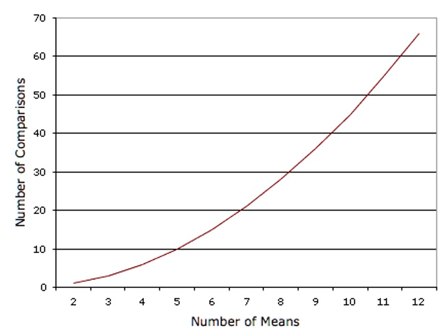
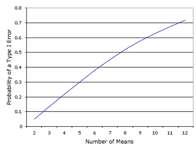
Figure 6.3 shows the probability of a Type I error as a function of the number of means. As you can see, if you have an experiment with 12 means, the probability is about 0.70 that at least one of the 66 comparisons among means would be significant even if all 12 population means were the same.
The collective Type I error rate can be controlled using various methods such as the Tukey Honestly Significant Difference test or Tukey HSD for short. The Tukey HSD test is one example of a multiple comparison test or adjustment, but several alternatives are frequently used, such as the Bonferroni correction and the Benjamini–Hochberg procedure. All approaches will make it more difficult to find statistical significance and thereby reduce the Type I error rate. There is ongoing debate on whether, how, and in what circumstances to adjust for multiple comparisons, so you are likely to encounter a variety of approaches when reading applied research reports.11
The Tukey HSD is based on a variation of the t distribution that takes into account the number of means being compared. This distribution is called the studentized range distribution.
Normally, statistical software will make all the necessary calculations for you in the background. But to illustrate what sorts of calculations the software is relying on, let’s return to the leniency study to see how to compute the Tukey HSD test. You will see that the computations are very similar to those of an independent-groups t test. The steps are outlined below:
- Compute the means and variances of each group. For our example, they are shown in Table 6.7.
| Condition | Mean | Variance | ||||
|---|---|---|---|---|---|---|
| False | 5.37 | 3.34 | ||||
| Felt | 4.91 | 2.83 | ||||
| Miserable | 4.91 | 2.11 | ||||
| Neutral | 4.12 | 2.32 |
Compute MSE, which is simply the mean of the variances. It is equal to 2.65.
Compute Q (using the formula below) for each pair of means, where \(\bar{X}_i\) is one mean, \(\bar{X}_j\) is the other mean, and \(n\) is the number of scores in each group. For these data, there are 34 observations per group. The value in the denominator is 0.279. \[ Q=\frac{\bar{X}_i-\bar{X}_j}{\sqrt{\frac{MSE}{n}}} \]
Compute p for each comparison using a Studentized Range Calculator.12 The degrees of freedom is equal to the total number of observations minus the number of means. For this experiment, df = 136 - 4 = 132.
The tests for these data are shown in Table 6.8.
| Comparison | \(\bar{X}_i - \bar{X}_j\) | \(Q\) | \(p\) |
|---|---|---|---|
| False - Felt | 0.46 | 1.65 | 0.649 |
| False - Miserable | 0.46 | 1.65 | 0.649 |
| False - Neutral | 1.25 | 4.48 | 0.010 |
| Felt - Miserable | 0.00 | 0.00 | 1.000 |
| Felt - Neutral | 0.79 | 2.83 | 0.193 |
| Miserable - Neutral | 0.79 | 2.83 | 0.193 |
The only significant comparison is between the false smile and the neutral smile.
It is not unusual to obtain results that on the surface appear paradoxical. For example, these results appear to indicate that (a) the false smile is the same as the miserable smile, (b) the miserable smile is the same as the neutral control, and (c) the false smile is different from the neutral control. This apparent contradiction is avoided if you are careful not to accept the null hypothesis when you fail to reject it. The finding that the false smile is not significantly different from the miserable smile does not mean that they are really the same. Rather it means that there is not convincing evidence that they are different. Similarly, the non-significant difference between the miserable smile and the control does not mean that they are the same. The proper conclusion is that the false smile is higher than the control and that the miserable smile is either (a) equal to the false smile, (b) equal to the control, or (c) somewhere in-between.
6.10 Chapter 6 Appendix II: Chi Square Tests13
A Chi Square test is so-named because it relies on a probability distribution called the Chi Square distribution (more details are beyond the scope of this text and can be found elsewhere14).
The first step is to compute the expected frequency for each cell based on the assumption that there is no relationship. These expected frequencies are computed from the totals as follows. We begin by computing the expected frequency for the AHA Diet-Cancers combination. Note that 22/605 subjects developed cancer. The proportion who developed cancer is therefore 0.0364. If there were no relationship between diet and outcome (as the null hypothesis states), then we would expect 0.0364 of those on the AHA diet to develop cancer. Since 303 subjects were on the AHA diet, we would expect (0.0364)(303) = 11.02 cancers on the AHA diet. Similarly, we would expect (0.0364)(302) = 10.98 cancers on the Mediterranean diet. In general, the expected frequency for a cell in the \(i\)th row and the \(j\)th column is equal to
\[ E_{ij}=\frac{T_iT_j}{T} \]
where \(E_{ij}\) is the expected frequency for cell \(i,j\), \(T_i\) is the total for the \(i\)th row, \(T_j\) is the total for the \(j\)th column, and \(T\) is the total number of observations. For the AHA Diet-Cancers cell, \(i = 1\), \(j = 1\), \(T_i = 303\), \(T_j = 22\), and \(T = 605\). Table 6.9 shows the expected frequencies (in parenthesis) for each cell in the experiment.
The significance test is conducted by computing Chi Square as follows.
\[ \chi^2_3=\sum\frac{(E-O)^2}{E}=16.55 \]
The degrees of freedom is equal to \((r-1)(c-1)\), where \(r\) is the number of rows and \(c\) is the number of columns. For this example, the degrees of freedom is \((2-1)(4-1) = 3\). A Chi Square calculator15 can be used to determine that the probability value for a Chi Square of 16.55 with three degrees of freedom is equal to 0.0009. Therefore, the null hypothesis of no relationship between diet and outcome can be rejected.
| Outcome | ||||
|---|---|---|---|---|
| Diet | Cancers | Fatal Heart Disease | Non-Fatal Heart Disease | Healthy |
| AHA | 15 (11.02) |
24 (19.03) |
25 (16.53) |
239 (256.42) |
| Mediterranean | 7 (10.98) |
14 (18.97) |
8 (16.47) |
273 (255.58) |
| Total | 22 | 38 | 33 | 512 |
Data shared under ODC-BY 1.0: Bonica, Adam. 2024. Database on Ideology, Money in Politics, and Elections: Public version 4.0 [Computer file]. Stanford, CA: Stanford University Libraries. https://data.stanford.edu/dime.↩︎
This description of “no relationship” is confined to a specific measure of association. For example, the null hypothesis might indicate no linear relationship between two variables (a correlation of zero) but say nothing about possibilities for a nonlinear relationship. Or it might indicate that the means are equal, saying nothing about medians or variances.↩︎
https://www2.census.gov/geo/pdfs/maps-data/maps/reference/us_regdiv.pdf↩︎
Rainey, C. (2014). Arguing for a negligible effect. American Journal of Political Science, 58(4), 1083-1091. https://doi.org/10.1111/ajps.12102↩︎
Gelman, A., & Stern, H. (2006). The difference between “significant” and “not significant” is not itself statistically significant. The American Statistician, 60(4), 328-331. https://doi.org/10.1198/000313006X152649↩︎
“All Pairwise Comparisons Among Means.” https://onlinestatbook.com/2/tests_of_means/pairwise.html↩︎
When discussing probability of Type I errors, we assume all null hypotheses are true, since a Type I error can’t occur if the null hypothesis is false.↩︎
García-Pérez, M. A. (2023). Use and misuse of corrections for multiple testing. Methods in Psychology, 8, 100120. https://doi.org/10.1016/j.metip.2023.100120↩︎
https://onlinestatbook.com/2/calculators/studentized_range_dist.html↩︎
This section is adapted from David M. Lane. “Contingency Tables.” Online Statistics Education: A Multimedia Course of Study. https://onlinestatbook.com/2/chi_square/contingency.html↩︎
For example, see David M. Lane. “Chi Square Distribution.” Online Statistics Education: A Multimedia Course of Study. https://onlinestatbook.com/2/chi_square/distribution.html↩︎
https://onlinestatbook.com/2/calculators/chi_square_prob.html↩︎