8 Sampling Distributions
Note: This chapter is adapted from the public domain resource Online Statistics Education: A Multimedia Course of Study (https://onlinestatbook.com Project Leader: David M. Lane, Rice University)
This is perhaps the most difficult chapter in the whole book. That is because sampling distributions are a very abstract concept that many students struggle to grasp. And yet sampling distributions are the core of how we conduct statistical inference. You may need to reread this chapter a few times before it makes much sense, but doing so will be well worth your time if you want to understand applied statistics.
8.1 Introduction to Sampling Distributions1
Suppose you randomly sampled 10 people from the population of women in Houston, Texas, between the ages of 21 and 35 years and computed the mean height of your sample. You would not expect your sample mean to be equal to the mean of all women in Houston. It might be somewhat lower or it might be somewhat higher, but it would not equal the population mean exactly. Similarly, if you took a second sample of 10 people from the same population, you would not expect the mean of this second sample to equal the mean of the first sample.
Recall from Chapter 5 that inferential statistics concern generalizing from a sample to a population (or to a counterfactual, but for this chapter we will focus on inferring about a population). A critical part of inferential statistics involves determining how far sample statistics are likely to vary from each other and from the population parameter being estimated. (In this example, the sample statistics are the sample means and the population parameter is the population mean.) As the later portions of this chapter show, these determinations are based on sampling distributions.
8.1.1 Discrete Distributions
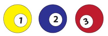
We will illustrate the concept of sampling distributions with a simple example. Figure 8.1 shows three pool balls, each with a number on it. Two of the balls are selected randomly (with replacement) and the average of their numbers is computed.
All possible outcomes are shown below in Table 8.1.
| Outcome | Ball 1 | Ball 2 | Mean | |||||
|---|---|---|---|---|---|---|---|---|
| 1 | 1 | 1 | 1.0 | |||||
| 2 | 1 | 2 | 1.5 | |||||
| 3 | 1 | 3 | 2.0 | |||||
| 4 | 2 | 1 | 1.5 | |||||
| 5 | 2 | 2 | 2.0 | |||||
| 6 | 2 | 3 | 2.5 | |||||
| 7 | 3 | 1 | 2.0 | |||||
| 8 | 3 | 2 | 2.5 | |||||
| 9 | 3 | 3 | 3.0 |
Notice that all the means are either 1.0, 1.5, 2.0, 2.5, or 3.0. The frequencies of these means are shown in Table 6-2. The relative frequencies are equal to the frequencies divided by nine because there are nine possible outcomes.
| Mean | Frequency | Relative Frequency | ||||
|---|---|---|---|---|---|---|
| 1.0 | 1 | 0.111 | ||||
| 1.5 | 2 | 0.222 | ||||
| 2.0 | 3 | 0.333 | ||||
| 2.5 | 2 | 0.222 | ||||
| 3.0 | 1 | 0.111 |
Figure 8.2 shows a relative frequency distribution of the means based on Table 8.2. This distribution is also a probability distribution since the y-axis is the probability of obtaining a given mean from a sample of two balls in addition to being the relative frequency.
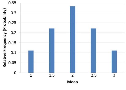
The distribution shown in Figure 8.2 is called the sampling distribution of the mean. Specifically, it is the sampling distribution of the mean for a sample size of 2 (n = 2). For this simple example, the distribution of pool balls and the sampling distribution are both discrete distributions. The pool balls have only the values 1, 2, and 3, and a sample mean can have one of only five values shown in Table 8.2.
There is an alternative way of conceptualizing a sampling distribution that will be useful for more complex distributions. Imagine that two balls are sampled (with replacement) and the mean of the two balls is computed and recorded. Then this process is repeated for a second sample, a third sample, and eventually thousands of samples. After thousands of samples are taken and the mean computed for each, a relative frequency distribution is drawn. The more samples, the closer the relative frequency distribution will come to the sampling distribution shown in Figure 8.2. As the number of samples approaches infinity, the relative frequency distribution will approach the sampling distribution. This means that you can conceive of a sampling distribution as being a relative frequency distribution based on a very large number of samples. To be strictly correct, the relative frequency distribution approaches the sampling distribution as the number of samples approaches infinity.
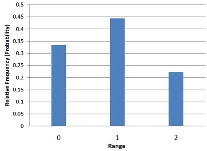
It is important to keep in mind that every statistic, not just the mean, has a sampling distribution. For example, Table 8.3 shows all possible outcomes for the range of two numbers (larger number minus the smaller number). Table 8.4 shows the frequencies for each of the possible ranges and Figure 8.3 shows the sampling distribution of the range.
| Outcome | Ball 1 | Ball 2 | Range | |||||
|---|---|---|---|---|---|---|---|---|
| 1 | 1 | 1 | 0 | |||||
| 2 | 1 | 2 | 1 | |||||
| 3 | 1 | 3 | 2 | |||||
| 4 | 2 | 1 | 1 | |||||
| 5 | 2 | 2 | 0 | |||||
| 6 | 2 | 3 | 1 | |||||
| 7 | 3 | 1 | 2 | |||||
| 8 | 3 | 2 | 1 | |||||
| 9 | 3 | 3 | 0 |
| Range | Frequency | Relative Frequency | ||||
|---|---|---|---|---|---|---|
| 0 | 3 | 0.333 | ||||
| 1 | 4 | 0.444 | ||||
| 2 | 2 | 0.222 |
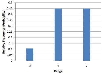
It is also important to keep in mind that there is a sampling distribution for various sample sizes. For simplicity, we have been using n = 2. The sampling distribution of the range for n = 3 is shown in Figure 8.4.
8.1.2 Continuous Distributions
In the previous section, the population consisted of three pool balls. Now we will consider sampling distributions when the population distribution is continuous. What if we had a thousand pool balls with numbers ranging from 0.001 to 1.000 in equal steps? (Although this distribution is not really continuous, it is close enough to be considered continuous for practical purposes.) As before, we are interested in the distribution of means we would get if we sampled two balls and computed the mean of these two balls. In the previous example, we started by computing the mean for each of the nine possible outcomes. This would get a bit tedious for this example since there are 1,000,000 possible outcomes (1,000 for the first ball x 1,000 for the second). Therefore, it is more convenient to use our second conceptualization of sampling distributions which conceives of sampling distributions in terms of relative frequency distributions. Specifically, the relative frequency distribution that would occur if samples of two balls were repeatedly taken and the mean of each sample computed.
When we have a truly continuous distribution, it is not only impractical but actually impossible to enumerate all possible outcomes. Moreover, in continuous distributions, the probability of obtaining any single value is zero. Therefore, these values are called probability densities rather than probabilities.
8.1.3 Sampling Distributions and Inferential Statistics
As we stated in the beginning of this chapter, sampling distributions are important for inferential statistics. In the examples given so far, a population was specified and the sampling distribution of the mean and the range were determined. In practice, the process proceeds the other way: you collect sample data and from these data you estimate parameters of the sampling distribution. This knowledge of the sampling distribution can be very useful. For example, knowing the degree to which means from different samples would differ from each other and from the population mean would give you a sense of how close your particular sample mean is likely to be to the population mean. Fortunately, this information is directly available from a sampling distribution. The most common measure of how much sample means differ from each other is the standard deviation of the sampling distribution of the mean. This standard deviation is called the standard error of the mean. If all the sample means were very close to the population mean, then the standard error of the mean would be small. On the other hand, if the sample means varied considerably, then the standard error of the mean would be large.
To be specific, assume your sample mean were 125 and you estimated that the standard error of the mean were 5 (using a method shown in a later section). If you had a normal distribution, then it would be likely that your sample mean would be within 10 units of the population mean since most of a normal distribution is within two standard deviations of the mean.
Keep in mind that all statistics have sampling distributions, not just the mean. For example, later in this chapter we will construct confidence intervals relying on the sampling distribution for a regression slope coefficient.
8.2 Sampling Distribution of the Mean2
As we learned in the prior section, the sampling distribution of the mean refers to the probability distribution describing all possible values of the sample mean we could obtain in repeated sampling. This section goes over some important properties of the sampling distribution of the mean.
8.2.1 Mean
The mean of the sampling distribution of the mean is the mean of the population from which the scores were sampled (or the expected value of the random data generating process). Therefore, if a population has a mean \(\mu\), then the mean of the sampling distribution of the mean (\(\bar{x}\)) is also \(\mu\). The symbol \(\mu_{\bar{x}}\) is used to refer to the mean of the sampling distribution of the mean. Therefore, the formula for the mean of the sampling distribution of the mean can be written as:
\[ \mu_{\bar{x}} = \mu \]
8.2.2 Variance
The variance of the sampling distribution of the mean is computed as follows:
\[ \sigma^2_{\bar{x}} = \frac{\sigma^2}{n} \]
That is, the variance of the sampling distribution of the mean is the population variance divided by \(n\), the sample size (the number of scores used to compute a mean).3 (If not sampling from a population, the variance of the probability distribution from which the random variable is drawn is used rather than the population variance.) Thus, the larger the sample size, the smaller the variance of the sampling distribution of the mean.
As noted previously, the standard error of the mean is the standard deviation of the sampling distribution of the mean. It is therefore the square root of the variance of the sampling distribution of the mean and can be written as:
\[ \sigma_{\bar{x}} = \frac{\sigma}{\sqrt{n}} \]
The standard error is represented by a \(\sigma\) because it is a standard deviation. The subscript (\(\bar{x}\)) indicates that the standard error in question is the standard error of the (sample) mean.
8.2.3 Central Limit Theorem
The central limit theorem states that:
Given a population with a finite mean \(\mu\) and a finite non-zero variance \(\sigma^2\), the sampling distribution of the mean approaches a normal distribution with a mean of \(\mu\) and a variance of \(\sigma^2/n\) as \(n\), the sample size, increases.
The expressions for the mean and variance of the sampling distribution of the mean are not new or remarkable. What is remarkable is that regardless of the shape of the parent population, the sampling distribution of the mean approaches a normal distribution as n increases. Figure 8.5 shows the results of the simulation for n = 2 and n = 10. The parent population was a uniform distribution. You can see that the distribution for n = 2 is far from a normal distribution. Nonetheless, it does show that the scores are denser in the middle than in the tails. For n = 10 the distribution is quite close to a normal distribution. Notice that the means of the two distributions are the same, but that the spread of the distribution for n = 10 is smaller.
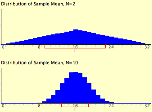
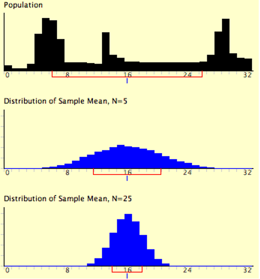
Figure 8.6 shows how closely the sampling distribution of the mean approximates a normal distribution even when the parent population is very non-normal. If you look closely you can see that the sampling distributions do have a slight positive skew. The larger the sample size, the closer the sampling distribution of the mean would be to a normal distribution.
8.3 Calculating Confidence Intervals
8.3.1 Confidence Intervals for the Mean4
When you compute a confidence interval on the mean, you compute the mean of a sample in order to estimate the mean of the population or the expected value. Clearly, if you already knew the population mean (expected value), there would be no need for a confidence interval. However, to explain how confidence intervals are constructed, we are going to work backwards and begin by assuming characteristics of the population. Then we will show how sample data can be used to construct a confidence interval.
8.3.1.1 An Artificial Example: Using the Normal Distribution
Assume that the weights of 10-year-old children are normally distributed with a mean of 90 and a standard deviation of 36. What is the sampling distribution of the mean for a sample size of 9? Recall from Section 8.2 that the mean of the sampling distribution is \(\mu\) and the standard error of the mean is
\[ \sigma_{\bar{x}} = \frac{\sigma}{\sqrt{n}} \]
For the present example, the sampling distribution of the mean has a mean of 90 and a standard deviation of 36/3 = 12. Note that the standard deviation of a sampling distribution is its standard error. Figure 8.7 shows this distribution. The shaded area represents the middle 95% of the distribution and stretches from 66.48 to 113.52. These limits were computed by adding and subtracting 1.96 standard deviations to/from the mean of 90 as follows:
\[ 90 - (1.96)(12) = 66.48 \]
\[ 90 + (1.96)(12) = 113.52 \]
The value of 1.96 is based on the fact that 95% of the area of a normal distribution is within 1.96 standard deviations of the mean (in Chapter 7, we used 2 as a close approximation, but 1.96 is a more precise value); 12 is the standard error of the mean given our sample size of 9.
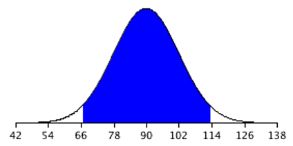
Figure 8.7 shows that 95% of the means are no more than 23.52 units (1.96 standard deviations) from the mean of 90. Now consider the probability that a sample mean computed in a random sample is within 23.52 units of the population mean of 90. Since 95% of the distribution is within 23.52 of 90, the probability that the mean from any given sample will be within 23.52 of 90 is 0.95. This means that if we repeatedly compute the mean (\(\bar{x}\)) from a sample (drawing a new random sample each time), and create an interval ranging from \(\bar{x} - 23.52\) to \(\bar{x} + 23.52\), this interval will contain the population mean 95% of the time. In general, you compute the 95% confidence interval for the mean with the following formula:
\[ \text{Lower limit} = \bar{x} - z_{.95}\times\sigma_{\bar{x}} \]\[ \text{Upper limit} = \bar{x} + z_{.95}\times\sigma_{\bar{x}} \]
where \(z_{.95}\) is the number of standard deviations extending from the mean of a normal distribution required to contain 0.95 of the area (always equal to 1.96) and \(\sigma_{\bar{x}}\) is the standard error of the mean.
If you look closely at this formula for a confidence interval, you will notice that you need to know the standard deviation (\(\sigma\)) in order to estimate the mean. This may sound unrealistic, and it is. However, computing a confidence interval when \(\sigma\) is known is easier than when \(\sigma\) has to be estimated, and serves a pedagogical purpose. Later in this section we will show how to compute a confidence interval for the mean when \(\sigma\) has to be estimated.
Suppose the following five numbers were sampled from a normal distribution with a standard deviation of 2.5: 2, 3, 5, 6, and 9. To compute the 95% confidence interval, start by computing the mean and standard error:
\[ \bar{x} = (2 + 3 + 5 + 6 + 9)/5 = 5. \]
\[ \sigma_{\bar{x}}=\frac{2.5}{\sqrt5}=1.118. \]
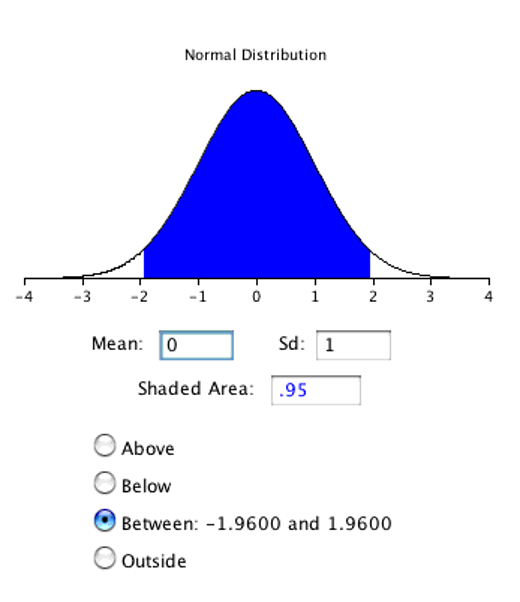
z.95 can be found using the normal distribution calculator5 and specifying that the shaded area is 0.95 and indicating that you want the area to be between the cutoff points. As shown in Figure 8.8, the value is 1.96. If you had wanted to compute the 99% confidence interval, you would have set the shaded area to 0.99 and the result would have been 2.58.
The 95% confidence interval can then be computed as follows:
\[ \text{Lower limit} = 5 - (1.96)(1.118)= 2.81 \]\[ \text{Upper limit} = 5 + (1.96)(1.118)= 7.19 \]
8.3.1.2 The Realistic Case: Using the T Distribution
You should use the t distribution rather than the normal distribution when the variance is not known and has to be estimated from sample data. You will learn more about the t distribution in the next section. When the sample size is large, say 100 or above, the t distribution is very similar to the standard normal distribution. However, with smaller sample sizes, the t distribution has relatively more scores in its tails than does the normal distribution. As a result, you have to extend farther from the mean to contain a given proportion of the area. Recall that with a normal distribution, 95% of the distribution is within 1.96 standard deviations of the mean. Using the t distribution, if you have a sample size of only 5, 95% of the area is within 2.78 standard deviations of the mean. Therefore, the standard error of the mean would be multiplied by 2.78 rather than 1.96.
The values of t to be used in a confidence interval can be looked up in a table of the t distribution, a small version of which is provided in the following section. You can also use an “inverse t distribution” calculator6 to find the t values to use in confidence intervals. With either approach, the t values will vary depending upon what is called the degrees of freedom (df). For confidence intervals on the mean, df is equal to n - 1, where n is the sample size.
Assume that the following five numbers are sampled from a normal distribution: 2, 3, 5, 6, and 9 and that the standard deviation is not known. The first steps are to compute the sample mean and variance:
\[ \bar{x} = 5 \]
\[ s^2 = 7.5 \]
The next step is to estimate the standard error of the mean. If we knew the population variance, we could use the following formula:
\[ \sigma_{\bar{x}} = \frac{\sigma}{\sqrt{n}} \]
Instead we compute an estimate of the standard error (\(s_{\bar{x}}\)). Note that since we previously computed the sample variance (\(s^2 = 7.5\)), we can take the square root of this to obtain the sample standard deviation (\(s\)):
\[ s_{\bar{x}} = \frac{s}{\sqrt{n}} = \frac{\sqrt{7.5}}{\sqrt{5}} = 1.225 \]
The next step is to find the value of t. As shown in Table 8.6 of the following section, the value for the 95% interval for df = n - 1 = 4 is 2.776. The confidence interval is then computed just as it is with \(\sigma_{\bar{x}}\). The only differences are that \(s_{\bar{x}}\) and \(t\) rather than \(\sigma_{\bar{x}}\) and \(z\) are used.
\[ \text{Lower limit} = 5 - (2.776)(1.225) = 1.60 \]\[ \text{Upper limit} = 5 + (2.776)(1.225) = 8.40 \]
More generally, the formula for the 95% confidence interval on the mean is:
\[ \text{Lower limit} = \bar{x} - (t_{CL})(s_{\bar{x}}) \]\[ \text{Upper limit} = \bar{x} + (t_{CL})(s_{\bar{x}}) \]
where \(\bar{x}\) is the sample mean, \(t_{CL}\) is the t for the confidence level desired (0.95 in the above example), and \(s_{\bar{x}}\) is the estimated standard error of the mean.
We will finish our discussion of confidence intervals for the mean with an analysis of the Stroop Data.7 Specifically, we will compute a confidence interval on the mean difference score. As mentioned in Section 2.5, the study involved 47 subjects naming the color of ink that words were written in. An additional detail that is now relevant to us is that subjects completed similar naming tasks multiple times under different conditions. In the “interference” condition, the names conflicted so that, for example, they would name the ink color of the word “blue” written in red ink. The correct response is to say “red” and ignore the fact that the word is “blue.” In a second condition, subjects named the ink color of colored rectangles.
| Naming Colored Rectangle | Interference | Difference | ||||
|---|---|---|---|---|---|---|
| 17 | 38 | 21 | ||||
| 15 | 58 | 43 | ||||
| 18 | 35 | 17 | ||||
| 20 | 39 | 19 | ||||
| 18 | 33 | 15 | ||||
| 20 | 32 | 12 | ||||
| 20 | 45 | 25 | ||||
| 19 | 52 | 33 | ||||
| 17 | 31 | 14 | ||||
| 21 | 29 | 8 |
Table 8.5 shows the time difference between the interference and color-naming conditions for 10 of the 47 subjects. The mean time difference for all 47 subjects is 16.362 seconds and the standard deviation is 7.470 seconds. The standard error of the mean is 1.090. A t table shows the critical value of t for 47 - 1 = 46 degrees of freedom is 2.013 (for a 95% confidence interval). Therefore the confidence interval is computed as follows:
\[ \text{Lower limit} = 16.362 - (2.013)(1.090) = 14.17 \]\[ \text{Upper limit} = 16.362 + (2.013)(1.090) = 18.56 \]
Therefore, the interference effect (difference) for the whole population is likely to be between 14.17 and 18.56 seconds.
8.3.2 More about the T Distribution8
In the introduction to normal distributions it was shown that 95% of the area of a normal distribution is within 1.96 standard deviations of the mean. Therefore, if you randomly sampled a value from a normal distribution with a mean of 100, the probability it would be within 1.96\(\sigma\) of 100 is 0.95. Similarly, if you sample n values from the population, the probability that the sample mean (\(\bar{x}\)) will be within 1.96 \(\sigma_{\bar{x}}\) of 100 is 0.95.
Now consider the case in which you have a normal distribution but you do not know the standard deviation. You sample \(n\) values and compute the sample mean (\(\bar{x}\)) and estimate the standard error of the mean (\(\sigma_{\bar{x}}\)) with \(s_{\bar{x}}\). What is the probability that \(\bar{x}\) will be within 1.96 \(s_{\bar{x}}\) of the population mean (\(\mu\))? This is a difficult problem because there are two ways in which \(\bar{x}\) could be more than 1.96 \(s_{\bar{x}}\) from \(\mu\): (1) \(\bar{x}\) could, by chance, be either very high or very low and (2) \(s_{\bar{x}}\) could, by chance, be very low. Intuitively, it makes sense that the probability of being within 1.96 standard errors of the mean should be smaller than in the case when the standard deviation is known (and cannot be underestimated). But exactly how much smaller? Fortunately, the way to work out this type of problem was solved in the early 20th century by W. S. Gosset who determined the distribution of a mean divided by an estimate of its standard error. This distribution is called the Student’s t distribution or sometimes just the t distribution. Gosset worked out the t distribution and associated statistical tests while working for a brewery in Ireland. Because of a contractual agreement with the brewery, he published the article under the pseudonym “Student.” That is why the t test is called the “Student’s t test.”
The t distribution is very similar to the normal distribution when the estimate of variance is based on a large sample, but the t distribution has relatively more scores in its tails when there is a small sample. When working with the t distribution, sample size is expressed in what are called degrees of freedom. Degrees of freedom indicate the number of independent pieces of information on which an estimate is based; a more complete discussion of the concept is provided in Appendix I at the end of this chapter. As we noted in the prior section, when we are estimating the standard error for a sample mean, the degrees of freedom is simply equal to the sample size minus one (n-1).
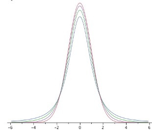
Figure 8.9 shows t distributions with 2, 4, and 10 degrees of freedom and the standard normal distribution. Notice that the normal distribution has relatively more scores in the center of the distribution and the t distribution has relatively more in the tails. The t distribution approaches the normal distribution as the degrees of freedom increase.
Since the t distribution has more area in the tails, the percentage of the distribution within 1.96 standard deviations of the mean is less than the 95% for the normal distribution. Table 8.6 shows the number of standard deviations from the mean required to contain 95% and 99% of the area of the t distribution for various degrees of freedom. These are the values of t that you use in a confidence interval. The corresponding values for the normal distribution are 1.96 and 2.58 respectively. Notice that with few degrees of freedom, the values of t are much higher than the corresponding values for a normal distribution and that the difference decreases as the degrees of freedom increase. The values shown in Table 6-7 can be obtained from statistical software or an online calculator.9
| df | 0.95 | 0.99 | ||||
| 2 | 4.303 | 9.925 | ||||
| 3 | 3.182 | 5.841 | ||||
| 4 | 2.776 | 4.604 | ||||
| 5 | 2.571 | 4.032 | ||||
| 8 | 2.306 | 3.355 | ||||
| 10 | 2.228 | 3.169 | ||||
| 20 | 2.086 | 2.845 | ||||
| 50 | 2.009 | 2.678 | ||||
| 100 | 1.984 | 2.626 |
Returning to the problem posed at the beginning of this section, suppose you sampled 9 values from a normal population and estimated the standard error of the mean (\(\sigma_{\bar{x}}\)) with \(s_{\bar{x}}\). What is the probability that \(\bar{x}\) would be within 1.96\(s_{\bar{x}}\) of \(\mu\)? Since the sample size is 9, there are n - 1 = 8 df. From Table 8.6, you can see that with 8 df the probability is 0.95 that the mean will be within 2.306 \(s_{\bar{x}}\) of \(\mu\). The probability that it will be within 1.96 \(s_{\bar{x}}\) of \(\mu\) is therefore lower than 0.95.
As shown in Figure 8.10, a t distribution calculator10 can be used to find that 0.086 of the area of a t distribution is more than 1.96 standard deviations from the mean, so the probability that \(\bar{x}\) would be less than 1.96\(s_{\bar{x}}\) from \(\mu\) is 1 - 0.086 = 0.914.
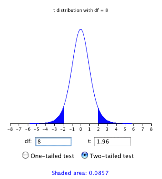
As expected, this probability is less than 0.95 that would have been obtained if \(\sigma_{\bar{x}}\) had been known instead of estimated.
8.3.3 Confidence Intervals for a Regression Slope Coefficient 11
The method for computing a confidence interval for the population slope in a simple linear regression is very similar to methods for computing other confidence intervals. For the 95% confidence interval, the formula is:
\[ \text{Lower limit} = \hat{\beta} - (t_{.95})(s_{\beta}) \]\[ \text{Upper limit} = \hat{\beta} + (t_{.95})(s_{\beta}) \]
where \(\hat{\beta}\) is the slope coefficient estimate, \(t_{.95}\) is the value of t for 95% (2-tailed) confidence, and \(s_{\beta}\) is the standard error for the slope estimate. As before, the t value can be found from a table or an inverse t distribution calculator based on the degrees of freedom.
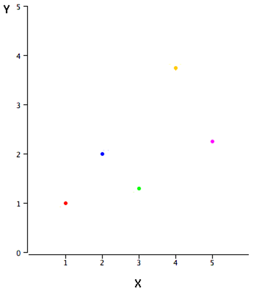
We illustrate generating a confidence interval using a very simple example with just five observations, depicted in Figure 8.11.
When conducting statistical inference for linear regression coefficients, the degrees of freedom is equal to the number of observations minus the number of coefficients being estimated (usually one for the intercept plus one for each independent variable). In the case of simple regression, there is just one independent variable plus a y-intercept, so the number of degrees of freedom is:
\[ df = n-2 \]
where \(n\) is the number of pairs of scores (number of observations in the sample).
The estimated regression slope coefficient is 0.425 with this data. An \(n\) of 5 yields 3 degrees of freedom (5 - 2 = 3), which means the critical t value (at 95% confidence) is 3.182. Finally, the estimated standard error for this slope coefficient (the calculative of which is shown in this chapter’s Appendix II) is 0.305 with this data.
Applying these formulas we obtain a confidence interval with the following lower and upper limits:
\[ \text{Lower limit} = 0.425 - (3.182)(0.305) = -0.55 \]\[ \text{Upper limit} = 0.425 + (3.182)(0.305) = 1.40 \]
8.4 Calcuating P-Values12
Now that we’ve learned about sampling distributions, we can fill in the details of how p-values are calculated. Let’s start by revisiting the first type of hypothesis test we encountered in this textbook: testing for the significance of a regression slope coefficient (Section 3.5).
The appropriate type of significance test in the case of the regression coefficients we have learned about is a t test. The general formula for computing a t statistic is:
\[ t = \frac{\text{point estimate - hypothesized value}}{\text{estimated standard error of point estimate}} \]
As applied to the case of the slope in a simple regression, the point estimate is the sample value of the slope coefficient (\(\hat{\beta}\)). The hypothesized value comes from our null hypothesis and is typically 0, meaning we want to test a null hypothesis of no relationship between the independent and dependent variables.
Just as when we generated a confidence interval for the slope coefficient in the prior section, the degrees of freedom for this t test is n-2. We also use the same calculation for the estimated standard error (again, see Appendix II).
With our example from the prior section, we had a sample slope coefficient (\(\hat{\beta}\)) of 0.425, an estimated standard error (\(s_{\beta}\)) of 0.305, and a sample size of 5. Given these numbers and a hypothesized value of 0:
\[ t = \frac{0.425-0}{0.305} = 1.39 \] \[ df = n-2 = 5-2 = 3. \]
From software or a t-distribution calculator, we find that with these values of \(t\) and \(df\), the two-tailed p-value is 0.26. Therefore, the slope is not significantly different from 0 under this example.
Appendix III provides further examples of how p-values are calculated, including for a one-tailed test. Details for other types of analysis can be found in various sources, including the free online text on which this chapter is based (difference of means, ANOVA, Chi Square tests)
8.5 Exercises13
A population has a mean of 50 and a standard deviation of 6. (a) What are the mean and standard deviation of the sampling distribution of the mean for N = 16? (b) What are the mean and standard deviation of the sampling distribution of the mean for N = 20?
What term refers to the standard deviation of the sampling distribution?
True/false: The standard error of the mean is smaller when N = 20 than when N = 10.
True/false: In your school, 40% of students watch TV at night. You randomly ask 5 students every day if they watch TV at night. Every day, you would find that 2 of the 5 do watch TV at night.
True/false: The median has a sampling distribution.
If the variable
xhas a population mean of 0 and a population standard deviation of 4 but is highly skewed, will the sampling distribution of the mean ofxapproach a normal distribution as the sample size increases?The exact shape of the t distribution changes depending on what parameter?
When is the t distribution virtually indistinguishable from the standard normal distribution?
With what sample size (small or large) is it especially important to use the t distribution rather than the normal distribution to calculate confidence intervals for a regression slope coefficient?
Suppose I am comparing two means (e.g., using regression) with a large sample size, and for the null hypotheses of equal means, I obtain a t-score of -3.4. What conclusion do I reach?
Chapter 8 Appendix I: Degrees of Freedom14
Some estimates are based on more information than others. For example, an estimate of the variance based on a sample size of 100 is based on more information than an estimate of the variance based on a sample size of 5. The degrees of freedom (df) of an estimate is the number of independent pieces of information on which the estimate is based.
As an example, let’s say that we know that the mean height of Martians is 6 and wish to estimate the variance of their heights. We randomly sample one Martian and find that its height is 8. Recall that the variance is defined as the mean squared deviation of the values from their population mean. We can compute the squared deviation of our value of 8 from the population mean of 6 to find a single squared deviation from the mean. This single squared deviation from the mean, (8-6)2 = 4, is an estimate of the mean squared deviation for all Martians. Therefore, based on this sample of one, we would estimate that the population variance is 4. This estimate is based on a single piece of information and therefore has 1 df. If we sampled another Martian and obtained a height of 5, then we could compute a second estimate of the variance, (5-6)2 = 1. We could then average our two estimates (4 and 1) to obtain an estimate of 2.5. Since this estimate is based on two independent pieces of information, it has two degrees of freedom. The two estimates are independent because they are based on two independently and randomly selected Martians. The estimates would not be independent if after sampling one Martian, we decided to choose its brother as our second Martian.
As you are probably thinking, it is pretty rare that we know the population mean when we are estimating the variance. Instead, we have to first estimate the population mean (\(\mu\)) with the sample mean (\(\bar{x}\)). The process of estimating the mean affects our degrees of freedom as shown below.
Returning to our problem of estimating the variance in Martian heights, let’s assume we do not know the population mean and therefore we have to estimate it from the sample. We have sampled two Martians and found that their heights are 8 and 5. Therefore \(\bar{x}\), our estimate of the population mean, is
\[ \bar{x} = (8+5)/2 = 6.5. \]
We can now compute two estimates of variance:
\[ \text{Estimate 1} = (8-6.5)^2 = 2.25 \]
\[ \text{Estimate 2} = (5-6.5)^2 = 2.25 \]
Now for the key question: Are these two estimates independent? The answer is no because each height contributed to the calculation of \(\bar{x}\). Since the first Martian’s height of 8 influenced \(\bar{x}\), it also influenced Estimate 2. If the first height had been, for example, 10, then \(\bar{x}\) would have been 7.5 and Estimate 2 would have been (5-7.5)2 = 6.25 instead of 2.25. The important point is that the two estimates are not independent and therefore we do not have two degrees of freedom. Another way to think about the non-independence is to consider that if you knew the mean and one of the scores, you would know the other score. For example, if one score is 5 and the mean is 6.5, you can compute that the total of the two scores is 13 and therefore that the other score must be 13-5 = 8.
In general, the degrees of freedom for an estimate is equal to the number of values minus the number of parameters estimated en route to the estimate in question. In the Martians example, there are two values (8 and 5) and we had to estimate one parameter (\(\mu\)) on the way to estimating the parameter of interest (\(\sigma^2\)). Therefore, the estimate of variance has 2 - 1 = 1 degree of freedom. If we had sampled 12 Martians, then our estimate of variance would have had 11 degrees of freedom. Therefore, the degrees of freedom of an estimate of variance is equal to n - 1, where n is the number of observations.
Recall from Section 2.4.4 that the formula for estimating the variance in a sample is:
\[ s^2=\frac{\sum_{i=1}^n {(x_i-\bar{x})^2}}{n-1} \]
The denominator of this formula is the degrees of freedom.
So far, we’ve mainly seen examples where the degrees of freedom is equal to n - 1. But as we saw in Section 8.3.3, the degrees of freedom can also be equal to other values such as n - 2. In the case of constructing a confidence interval for a coefficient from a multiple regression with four independent variables, the degrees of freedom will generally be equal to n - 5. The exact formula for degrees of freedom depends on what we are estimating.
Chapter 8 Appendix II: Estimating the Standard Error of a Regression Slope15
Note that in this appendix, I depart from my notation throughout the rest of the book by using uppercase letters (\(X\) and \(Y\)) to refer to our variables of interest, in order to allow for lowercase letters (\(x\) and \(y\)) to refer to a transformed (mean-centered) version of these variables. This will simplify some of the presentation of material.
This appendix shows how to compute the estimated standard error for the slope of a simple linear regression. The estimated standard error of \(\beta\) is computed using the following formula:
\[ s_{\beta} = \frac{s_{est}}{\sqrt{SSX}} \]
where \(s_{\beta}\) is the estimated standard error of \(\beta\), \(s_{est}\) is the standard error of the estimate, and \(SSX\) is the sum of squared deviations of \(X\) from the mean of \(X\). \(SSX\) is calculated as:
\[ SSX = \sum_{i=1}^n {(X_i-\bar{X})^2} \]
where \(\bar{X}\) is the mean of \(X\). The standard error of the estimate can be calculated as:
\[ s_{est} = \sqrt{\frac{(1-r^2)SSY}{n-2}} \]
where \(r\) is the correlation between \(X\) and \(Y\), and \(SSY\) is the sum of squared deviations of \(Y\) from the mean of \(Y\).
These formulas are illustrated with the data shown in Table 8.7. These data are the same as in the example from Section 8.3.3. The column X has the values of the independent variable and the column Y has the values of the dependent variable. The third column, x, contains the differences between the values of column X and the mean of X. The fourth column, x2, is the square of the x column. The fifth column, y, contains the differences between the values of column Y and the mean of Y. The last column, y2, is simply square of the y column.
| X | Y | x | x2 | y | y2 | |
|---|---|---|---|---|---|---|
| 1.00 | 1.00 | -2.00 | 4 | -1.06 | 1.1236 | |
| 2.00 | 2.00 | -1.00 | 1 | -0.06 | 0.0036 | |
| 3.00 | 1.30 | 0.00 | 0 | -0.76 | 0.5776 | |
| 4.00 | 3.75 | 1.00 | 1 | 1.69 | 2.8561 | |
| 5.00 | 2.25 | 2.00 | 4 | 0.19 | 0.0361 | |
| Sum | 15.00 | 10.30 | 0.00 | 10.00 | 0.00 | 4.5970 |
\(SSY\) is the sum of squared deviations from the mean of y. It is, therefore, equal to the sum of the y2 column and is equal to 4.597. The correlation (\(r\)) between \(X\) and \(Y\) is 0.6268, and there are 5 observations (n=5). Thus, the standard error of the estimate is:
\[ s_{est} = \sqrt{\frac{(1-(0.6268)^2)(4.597)}{5-2}} = \sqrt{\frac{2.791}{3}} = 0.964 \]
\(SSX\) can be found as the sum of the x2 column and is equal to 10.
We now have all the information to compute the standard error of \(\beta\):
\[ s_{\beta} = \frac{0.964}{\sqrt{10}} = 0.305 \]
Chapter 8 Appendix III: Testing a Single Mean16
The way we calculate the probability (\(p\)) value for a hypothesis test depends on what type of statement is made in our null hypothesis. Normally, statistical software will automatically compute a p value behind the scenes, but we still want to learn a bit about how the software comes up with this value. To illustrate what these calculations can look like, this section will focus on what to do if we want to test a null hypothesis stating that the population mean is equal to some hypothesized value. For example, suppose an experimenter wanted to know if people are influenced by a subliminal message and performed the following experiment. Each of nine subjects is presented with a series of 100 pairs of pictures, and for each pair they are asked to select one. As a pair of pictures is presented, a subliminal message is presented suggesting the picture that the subject should choose. The question is whether the (population) mean number of times the suggested picture is chosen is equal to 50 (the number we would expect if subliminal messages have no effect). In other words, the null hypothesis is that the population mean (\(\mu\)) is 50. The (hypothetical) data are shown in Table 8.8. The data in Table 8.8 have a sample mean (\(\bar{x}\)) of 51. Thus the sample mean differs from the hypothesized population mean by 1.
| Frequency |
|---|
| 45 |
| 48 |
| 49 |
| 49 |
| 51 |
| 52 |
| 53 |
| 55 |
| 57 |
The significance test consists of computing the probability of a sample mean differing from \(\mu\) by one (the difference between the hypothesized population mean and the sample mean) or more. The first step is to determine the sampling distribution of the mean. As we learned in the prior chapter, the mean and standard deviation of the sampling distribution of the mean are
\[ \mu_{\bar{x}} = \mu \]
and
\[ \sigma_{\bar{x}} = \frac{\sigma}{\sqrt{n}} \]
respectively. It is clear that if the null hypothesis is true, \(\mu_{\bar{x}}\) = 50. In order to compute the standard deviation of the sampling distribution of the mean, we have to know the population standard deviation (\(\sigma\)).
The current example was constructed to be one of the few instances in which the standard deviation is known. In practice, it is very unlikely that you would know \(\sigma\) and therefore you would use \(s\), the sample estimate of \(\sigma\). However, it is instructive to see how the probability is computed if \(\sigma\) is known before proceeding to see how it is calculated when \(\sigma\) is estimated.
For the current example, if the null hypothesis is true, then based on a well-established formula for the binomial distribution, one can compute that the variance of the number correct is
\[ \sigma^2 = N \pi (1-\pi) = 100(0.5)(1-0.5) = 25 \]
where \(N\) is the number of times a subject makes a selection between two pictures. Therefore, \(\sigma\) = 5 (since \(\sigma = \sqrt{\sigma^2}=\sqrt{25}=5\)). For a \(\sigma\) of 5 and an \(n\) of 9, the standard deviation of the sampling distribution of the mean is \(5/\sqrt{9} = 1.667\). Recall that the standard deviation of a sampling distribution is called the standard error.
To recap, we wish to know the probability of obtaining a sample mean of 51 or greater assuming the null hypothesis is true. If the null hypothesis is true, the sampling distribution of the mean has a mean of 50 and a standard deviation of 1.667. To compute the relevant probability, we will make the assumption that the sampling distribution of the mean is normally distributed. We can then use a normal distribution calculator as shown in Figure 8.12.
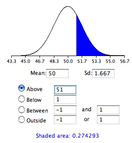
Notice that the mean is set to 50, the standard deviation to 1.667, and the area above 51 is requested and shown to be 0.274.
Therefore, the probability of obtaining a sample mean of 51 or larger is 0.274. Since a mean of 51 or higher is not unlikely under the assumption that the subliminal message has no effect, the effect is not significant and the null hypothesis is not rejected.
The test conducted above was a one-tailed test because it computed the probability of a sample mean being one or more points higher than the hypothesized mean of 50 and the area computed was the area above 51. To test the two-tailed hypothesis, you would compute the probability of a sample mean differing by one or more in either direction from the hypothesized mean of 50. You would do so by computing the probability of a mean being less than or equal to 49 or greater than or equal to 51.
The results from a normal distribution calculator are shown in Figure 8.13.
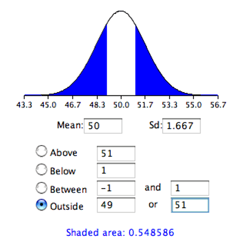
As you can see, the probability is 0.548 which, as expected, is twice the probability of 0.274 shown in Figure 8.12.
Before normal calculators such as the one illustrated above were widely available, probability calculations were made based on the standard normal distribution (which also maps to how we conduct t tests). This was done by computing \(z\) based on the formula
\[ z = \frac{\bar{x}-\mu_0}{\sigma_{\bar{x}}} \]
where \(z\) is the value on the standard normal distribution, \(\bar{x}\) is the sample mean, \(\mu_0\) is the hypothesized value of the mean (under the null hypothesis),17 and \(\sigma_{\bar{x}}\) is the standard error of the mean. For this example, \(z\) = (51-50)/1.667 = 0.60. Use a normal calculator, with a mean of 0 and a standard deviation of 1, as shown below.
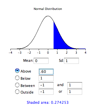
Notice that the probability (the shaded area) is the same as previously calculated (for the one-tailed test).
As noted, in real-world data analyses it is very rare that you would know \(\sigma\) and wish to estimate \(\mu\). Typically \(\sigma\) is not known and is estimated in a sample by s, and \(\sigma_{\bar{x}}\) is estimated by \(s_{\bar{x}}\). For our next example, we will consider the data in the “ADHD Treatment” case study.18 These data consist of the scores of 24 children with ADHD on a delay of gratification (DOG) task. Each child was tested under four dosage levels. Table 8.9 shows the data for the placebo (0 mg) and highest dosage level (0.6 mg) of methylphenidate. Of particular interest here is the column labeled “Diff” that shows the difference in performance between the 0.6 mg (D60) and the 0 mg (D0) conditions. These difference scores are positive for children who performed better in the 0.6 mg condition than in the control condition and negative for those who scored better in the control condition. If methylphenidate has a positive effect, then the mean difference score in the population will be positive. The null hypothesis is that the mean difference score in the population is 0.
| D0 | D60 | Diff | ||||
|---|---|---|---|---|---|---|
| 57 | 62 | 5 | ||||
| 27 | 49 | 22 | ||||
| 32 | 30 | -2 | ||||
| 31 | 34 | 3 | ||||
| 34 | 38 | 4 | ||||
| 38 | 36 | -2 | ||||
| 71 | 77 | 6 | ||||
| 33 | 51 | 18 | ||||
| 34 | 45 | 11 | ||||
| 53 | 42 | -11 | ||||
| 36 | 43 | 7 | ||||
| 42 | 57 | 15 | ||||
| 26 | 36 | 10 | ||||
| 52 | 58 | 6 | ||||
| 36 | 35 | -1 | ||||
| 55 | 60 | 5 | ||||
| 36 | 33 | -3 | ||||
| 42 | 49 | 7 | ||||
| 36 | 33 | -3 | ||||
| 54 | 59 | 5 | ||||
| 34 | 35 | 1 | ||||
| 29 | 37 | 8 | ||||
| 33 | 45 | 12 | ||||
| 33 | 29 | -4 |
To test this null hypothesis, we compute what we call a t statistic (as opposed to a z statistic) because we will compare this value to the t distribution—a distribution which allows for accurate inferences when \(\sigma\) is estimated rather than known (see Section 8.3.2). We compute t using a special case of the following formula:
\[ \text{t} = \frac{\text{point estimate} -\text{hypothesized value}}{\text{estimated standard error of point estimate}} \]
The special case of this formula applicable to testing a single mean is
\[ \text{t} = \frac{\bar{x}-\mu_0}{s_{\bar{x}}} \]
where \(t\) is the value we compute for the significance test, \(\bar{x}\) is the sample mean, \(\mu_0\) is the hypothesized value of the population mean, and \(s_{\bar{x}}\) is the estimated standard error of the mean. Notice the similarity of this formula to the formula for \(z\) we saw before.
In the previous example, we assumed that the scores were normally distributed. In this case, it is the population of difference scores that we assume to be normally distributed.
The mean (\(\bar{x}\)) of the n = 24 difference scores is 4.958, the hypothesized value of \(\mu\) is 0, and the standard deviation (s) is 7.538. The estimate of the standard error of the mean is computed as:
\[ s_{\bar{x}} = \frac{s}{\sqrt{n}} = \frac{7.5382}{\sqrt{24}} = 1.54 \]
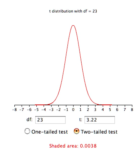
Therefore, t = 4.96/1.54 = 3.22. The probability value for t depends on the degrees of freedom. The number of degrees of freedom is equal to n - 1 = 23. As shown below, a t distribution calculator finds that the probability of a t less than -3.22 or greater than 3.22 is only 0.0038. Therefore, if the drug had no effect, the probability of finding a difference between means as large or larger (in either direction) than the difference found is very low. Therefore the null hypothesis that the population mean difference score is zero can be rejected. The conclusion is that the population mean for the drug condition is higher than the population mean for the placebo condition.
In order to conduct this hypothesis test, we made the following assumptions:
Each value is sampled independently from each other value.
The values are sampled from a normal distribution.
This subsection is adapted from David M. Lane. “Introduction to Sampling Distributions.” Online Statistics Education: A Multimedia Course of Study. https://onlinestatbook.com/2/sampling_distributions/intro_samp_dist.html↩︎
This subsection is adapted from David M. Lane. “Sampling Distribution of the Mean.” Online Statistics Education: A Multimedia Course of Study. https://onlinestatbook.com/2/sampling_distributions/samp_dist_mean.html↩︎
This expression can be derived very easily from the variance sum law. Let’s begin by computing the variance of the sampling distribution of the sum of three numbers sampled from a population with variance \(\sigma^2\). The variance of the sum would be \(\sigma^2 + \sigma^2 + \sigma^2\). For \(n\) numbers, the variance would be \(n\sigma^2\). Since the mean is \(1/n\) times the sum, the variance of the sampling distribution of the mean would be \(1/n^2\) times the variance of the sum, which equals \(\sigma^2/n\).↩︎
This subsubsection is adapted from David M. Lane. “Confidence Interval on the Mean.” Online Statistics Education: A Multimedia Course of Study. https://onlinestatbook.com/2/estimation/mean.html↩︎
https://onlinestatbook.com/2/calculators/inverse_t_dist.html↩︎
This section is adapted from David M. Lane. “t Distribution.” Online Statistics Education: A Multimedia Course of Study. https://onlinestatbook.com/2/estimation/t_distribution.html↩︎
https://onlinestatbook.com/2/calculators/inverse_t_dist.html↩︎
This section is adapted from David M. Lane. “Inferential Statistics for b and r.” Online Statistics Education: A Multimedia Course of Study. https://onlinestatbook.com/2/regression/inferent↩︎
This section is adapted from David M. Lane. “Inferential Statistics for b and r.” Online Statistics Education: A Multimedia Course of Study. https://onlinestatbook.com/2/regression/inferent↩︎
Questions 1-5 adapted from David M. Lane. “Exercises.” Online Statistics Education: A Multimedia Course of Study. https://onlinestatbook.com/2/sampling_distributions/ch7_exercises.html↩︎
This section is adapted from David M. Lane. “Degrees of Freedom.” Online Statistics Education: A Multimedia Course of Study. https://onlinestatbook.com/2/estimation/df.html↩︎
This section is adapted from David M. Lane. “Inferential Statistics for b and r.” Online Statistics Education: A Multimedia Course of Study. https://onlinestatbook.com/2/regression/inferent↩︎
This section is adapted from David M. Lane. “Testing a Single Mean.” Online Statistics Education: A Multimedia Course of Study. https://onlinestatbook.com/2/tests_of_means/single_mean.html↩︎
The subscript \(_0\) in \(\mu_0\) (the population mean according to the null hypothesis) corresponds to how we typically represent the null hypothesis: \(H_0\).↩︎