11  Regression Models

Regression is the most important tool for statistical analysis in the social sciences, and we have already seen several examples of how regression is used, starting from Section 3.4. In this chapter, we will learn more about the assumptions that typically underlie our regression models as well as how we can think about using regression to test more complex relationships among variables than we have examined so far.

11.1 Regression Assumptions

There are many different articulations of the assumptions that underlie our typical linear regression models, with some authors providing longer lists than others. Here, we will focus on the list provided by Gelman, Hill, and Vehtari (2021), which has the benefit of being arranged in decreasing order of importance. The authors caution, though, that this list of assumptions is for predictive inferences; drawing causal conclusions requires additional considerations, as implied by the discussion of causality in Chapter 9.

1. Validity

Just as our list of Three Questions to Always Ask about Data prods us to start by asking “what is being measured?”, the first regression assumption highlights the importance of valid measurement of variables (see discussion of validity in Chapter 10). With any statistical analysis (whether using regression or not), the data in the sample must validly measure whatever you are trying to understand, or else the results will be of no use. In their concept of validity, Gelman and colleagues also indicate the need to “include all relevant” independent variables and to have observations that fall within the realm of the phenomena of interest (e.g., a study of employee attitudes should use a sample that consists of employees). Deciding on which independent variables to include in a regression will be discussed in more detail in Section 11.2.

2. Representativeness

The data should be appropriate for generalizing to the broader phenomena of interest (external validity). As a simple example, a representative sample from a population (as would be found in expectation under random sampling) meets this assumption. It is not always necessary to have a perfectly representative sample to draw valid conclusions about associations, so long as the associations among variables are the same in the sample as in the population. For example, a sample that overrepresents young people could potentially yield accurate estimates of the association between exercise and happiness in the general population, so long as the exercise-happiness relationship plays out similarly among older and younger people. It is also the case that we are not always studying a well defined population. Thus, we sometimes need to interpret this assumption as indicating that the observations in the sample are representative instances of whatever it is we care to learn about (even if that phenomena of interest is not easily defined as a population).

3. Additivity and linearity

We use the term “linear regression” to refer to the standard regression model because of its linear form: the value of each independent variable is multiplied by a constant, and then these products are added up to form the predicted value of the dependent variable (together with the intercept). We will see this written out as an equation in Section 11.2. Predictions from a linear regression model will always follow this pattern of additivity and linearity. If we wish to create predictions that cannot be represented through a linear combination of independent variables, a linear regression is the wrong tool to use. Note, however, that sometimes relationships that are not strictly linear can still be approximated through a linear function. Linear relationships offer a simplicity that is not always apparent in other functional forms, so sometimes we may prefer the straightforward interpretability of linear regression results at the cost of the flexibility we might be able to achieve with other types of models. For example, if our primary concern is whether two variables generally exhibit a positive (versus negative) association and what the general strength of that association is, we may prefer a linear model of that association since it can provide a single number (a slope coefficient) that indicates direction and magnitude of association, even if this number oversimplifies a bit (as when there is some curvature in the true line describing their association).

Another important consideration to mention here (that we will explore in more detail later on in this chapter, and in the next) is that certain non-linear relationships can be modeled through linear regression, so long as they can be expressed by manipulating variables to create a linear function that represents these non-linearities. For example, the relationship between two variables need not follow a straight line if we transform the independent variable by squaring it, allowing for a prediction line to follow the shape of a parabola (for the original, untransformed variable).

If an independent variable is binary, the assumption of linearity is not practically restrictive. Since binary variables can only take on two different values (typically coded as 0 and 1), the coefficient associated with a binary variable will simply indicate how much to shift the prediction when going from one value to the other. The shape of the “line” connecting the two points is immaterial. Thus, linear regression can generally be considered “non-parametric” (meaning minimal assumptions are imposed) when studying only binary independent variables. In such cases, we can think of regression as simply using an equation to compare means across groups, as discussed in Chapter 4 and Chapter 6.

4. Independence of errors

The “errors” referred to in this list of assumptions come from the error term in a regression model, as introduced in Section 7.2. This fourth assumption implies that each observation in the sample represents a truly unique datapoint compared to all the others, at least when it comes to the value of the error term. Because the social world is full of interconnections, we often see violations of this assumption. Suppose, for example, that customer attitudes are measured using a survey of 1000 customers collected at 20 different restaurants. Though there is a sample size of 1000, each of the 20 restaurants may have its own peculiaries that shape customer attitudes in particular ways. Thus, the errors of prediction for the individuals may be interrelated (rather than fully independent) within each restaurant.¹

Fortunately, there are several techniques that can help us adjust our regression models to accommodate non-independence of errors, so long as we can accurately identify the structure(s) by which observations’ errors are interrelated.² The simplest structure is when we can group observations into mutually exclusive “clusters,” as in the case of the restaurant example above. There are multiple techniques that can adjust our regression estimates for such clustering, with the simplest being to make adjustments to our standard error estimates using one of several techniques known as “cluster robust standard errors.” Most statistical software packages will easily allow you to implement estimation of such standard errors. More advanced (and flexible) approaches to dealing with clustered observations can be found using tools from multi-level modeling.³

Another setting where we often adjust for violations of this assumption is when we are analyzing panel (or time series) data. Since the same units (e.g., individuals or organizations) are being observed multiple times within a dataset, observations are not expected to be fully independent of one another (e.g., an individual with above-average satisfaction in one time period will likely continue to be fairly satisfied in the following period). A variety of techniques have been developed to address concerns associated with the non-independence of errors when working with panel (or time series) data, and effectively working with such data will typically require serious study of such techniques.

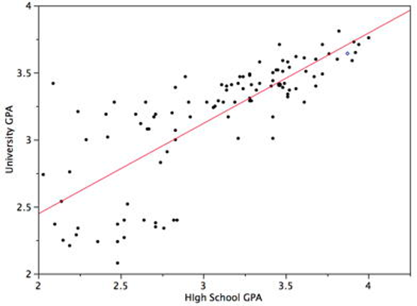
5. Equal variance of errors⁴

This assumption, known as homoskedasticity, indicates that the variance around the regression line is the same for all values of the independent variable(s). A clear violation of this assumption is shown in Figure 11.1. Notice that the predictions for students with high high-school GPAs are very good, whereas the predictions for students with low high-school GPAs are not very good. In other words, the points for students with high high-school GPAs are close to the regression line, whereas the points for low high-school GPA students are not.

Figure 11.1: University GPA as a function of High School GPA.

When errors have unequal variance, we call this heteroskedasticity. A common solution (easily implemented in most statistical software) is to calculate standard errors that are robust to heteroskedasticity. Some analysts will default to always using heteroskedastic-robust standard errors, although such corrections do not always work well in small samples.⁵

6. Normality of errors

This assumption is considered to the be least important. Still, regression results can sometimes become unreliable or imprecise when the distribution of errors has excessive outliers that are associated with certain non-normal distributions. This is particularly true when working with small samples. Thus, it can be useful to check variables for outliers, as well as examining the distribution of the residuals (estimated values of the error term in a regression model), which can easily be obtained in statistical software. Robust versions of regression are readily available in most statistical software and should be less vulnerable to problems created by violations of the normality assumption.⁶

11.2 Multiple Regression⁷

In simple linear regression, a dependent variable is predicted from one independent variable. In multiple regression, the dependent variable is predicted by two or more variables. For example, in the SAT case study we’ve used several times already to illustrate regression, you might want to predict a student’s university grade point average on the basis of their High-School GPA (HSGPA) and their total SAT score (verbal + math). The basic idea is to find a linear combination⁸ of HSGPA and SAT that best predicts University GPA (UGPA). That is, the problem is to find the values of \(\beta_1\) and \(\beta_2\) in the equation shown below that give the best predictions of UGPA. As in the case of simple linear regression, we define the best predictions as the predictions that minimize the squared errors of prediction (the “least squares” criterion).

\[\widehat{UGPA}_i = \alpha + \beta_1HSGPA_i + \beta_2SAT_i\]

where \(\widehat{UGPA}\) is the predicted value of University GPA and \(\alpha\) is the intercept (note that many authors instead use \(\beta_0\) to denote the intercept). For these data, the best prediction equation is shown below:

\[\widehat{UGPA}_i = 0.540 + 0.541 \times HSGPA_i + 0.008 \times SAT_i \tag{11.1}\]

In other words, to compute the prediction of a student’s University GPA, you add up (a) 0.540, (b) their High-School GPA multiplied by 0.541, and (c) their SAT multiplied by 0.008.

For comparison purposes, here is the regression equation from the simple regression discussed in Section 3.4.

\[ \widehat{UGPA}_i = 1.097 + 0.675 \times HSGPA_i \tag{11.2}\]

Table 11.1 shows the data and predictions for the first five students in the dataset based on the multiple regression (Equation 11.1).

Table 11.1: Data and Predictions

	\(HSGPA\)		\(SAT\)		\(\widehat{UGPA}\)
	3.45		1232		3.38
	2.78		1070		2.89
	2.52		1086		2.76
	3.67		1287		3.55
	3.24		1130		3.19

The values of \(\beta\) (\(\beta_1\) and \(\beta_2\)) are called “regression slope coefficients.”

The multiple correlation (R) is equal to the correlation between the predicted scores and the actual scores. In this example, it is the correlation between \(\widehat{UGPA}\) and \(UGPA\), which turns out to be 0.79. That is, R = 0.79. Note that R will never be negative since if there are negative correlations between the predictor variables and the criterion, the regression coefficients will be negative so that the correlation between the predicted and actual scores will be positive. By squaring the value of R, we obtain the commonly reported R-squared statistic (also written r^2 or \(R^2\)). R-squared indicates the proportion of variation in the dependent variable that can be explained by the independent variables in the model (or put differently, the proportion of variance in the dependent variable accounted for by the predicted scores).

Interpretation of Regression Coefficients

A regression coefficient in multiple regression is the slope of the linear relationship between the criterion variable and the part of a predictor variable that is independent of all other predictor variables. There are multiple ways to explain this computation, with additional descriptions provided in the appendix. As one approach, the regression coefficient for HSGPA can be computed by first predicting HSGPA from SAT and saving the errors of prediction (the differences between \(HSGPA\) and \(\widehat{HSGPA}\)). These errors of prediction are called “residuals” since they are what is left over in HSGPA after the predictions from SAT are subtracted, and represent the part of HSGPA that is independent of SAT. These residuals are referred to as HSGPA.SAT, which means they are the residuals in HSGPA after having been predicted by SAT. The correlation between HSGPA.SAT and SAT is necessarily 0.

The final step in computing the regression coefficient is to find the slope of the relationship between these residuals and UGPA. This slope is the regression coefficient for HSGPA. The following equation is used to predict HSGPA from SAT:

\[\widehat{HSGPA}_i = -1.314 + 0.0036 \times SAT_i\]

The residuals are then computed as:

\[HSGPA.SAT_i = HSGPA_i - \widehat{HSGPA}_i\]

The linear regression equation for the prediction of UGPA by the residuals is

\[\widehat{UGPA}_i = 3.173 + 0.541 \times HSGPA.SAT_i\]

Notice that the slope (0.541) is the same value given previously for the estimate of \(\beta_1\) in the multiple regression equation.

This means that the regression coefficient for HSGPA is the slope of the relationship between the dependent variable and the part of HSGPA that is independent of (uncorrelated with) the other independent variables. It represents the change in the prediction for the dependent variable associated with a change of one in the independent variable when all other independent variables are held constant. Since the regression coefficient for HSGPA is 0.54, this means that, holding SAT constant, a change of one in HSGPA is associated with a change of 0.54 in \(\widehat{UGPA}\). If two students had the same SAT and differed in HSGPA by 2, then you would predict they would differ in UGPA by (2)(0.54) = 1.08. Similarly, if they differed by 0.5, then you would predict they would differ by (0.50)(0.54) = 0.27.

The slope of the relationship between the dependent variable and the part of an independent variable that is unique from (independent of) other independent variables is its partial slope. Thus, the regression coefficient of 0.541 for HSGPA and the regression coefficient of 0.008 for SAT are partial slopes. Each partial slope represents the relationship between the independent variable and the dependent variable holding constant all of the other independent variables.

It is difficult to compare the coefficients for different variables directly because they are measured on different scales. A difference of 1 in HSGPA is a fairly large difference, whereas a difference of 1 on the SAT is negligible. Therefore, it can be advantageous to transform the variables so that they are on the same scale. The most straightforward approach is to standardize the variables (see Section 2.6.1) so that they each have a standard deviation of 1. A regression coefficient for standardized variables is called a “standardized coefficient” or “beta coefficient.” For these data, the standardized coefficients are 0.625 and 0.198. These values represent the change in the prediction for the dependent variable (in standard deviations) associated with a change of one standard deviation on an independent variable (holding constant the value(s) on the other independent variable(s)). Clearly, a change of one standard deviation on HSGPA is associated with a larger difference than a change of one standard deviation of SAT. In practical terms, this means that if you know a student’s HSGPA, knowing the student’s SAT does not aid the prediction of UGPA much. However, if you do not know the student’s HSGPA, his or her SAT can aid in the prediction since the standardized coefficient in the simple regression predicting UGPA from SAT is 0.68. For comparison purposes, the standardized coefficient in the simple regression predicting UGPA from HSGPA is 0.78. As is typically the case, the partial slopes are smaller than the slopes in simple regression.

11.2.1 Deciding Which Independent Variables to Include⁹

It is a bit hard to generalize regarding the criteria for deciding which varaibles to include as independent variables, because it depends on the research question posed and whether the goal is to describe general patterns of association, to identify a predictive relationship, or to identify a causal or possibly causal relationship.

To help guide our discussion of variable selection, we will distinguish between key independent variables of interest (those that the analyst is particularly interested in learning about) and control variables. We will represent the former using X and the latter as Z. When we add an independent variable Z to a regression not because we are particularly interested in estimating the association of Z with the dependent variable Y but instead because we think including Z in the regression will yield better estimates for how X is associated with Y, we often refer to Z as a control variable. Control variables are not different from independent variables, as far as the statistical estimation is concerned. They are merely different labels that signal a difference in the researcher’s substantive interest in the slope coefficients for these variables (e.g., control variables are probably not the subjects of any hypotheses).

Obviously, any variable X of substantive interest should be included in a regression, although it is sometimes beneficial to include various X variables one at a time if one is not interested in describing how each one relates to to Y independent of the other X variables.

Where the interest lies (at least to some extent) in considering causal relationships among variables, you should generally include potential confounders to the X-Y relationship as control variables (additional independent variables) in a regression.

You might also consider including as a control variable any factor that you believe will be a strong cause of the dependent variable, so long as this factor is not itself caused by X. Adding such variables will generally improve the precision of our estimates (making standard errors smaller).

When there is an interest in causal relationships, it is generally best to avoid adding as control variables anything that may be caused by X. One reason is that when X causes Z and Z causes Y, Z is a mediator, and therefore Z is one route (or mechanism) through which X may affect Y. Thus, by controlling for (or pulling out) one route through which X may affect Y, we are distorting our ability to observe the total effect of X on Y.

For estimations of causal effects, a more complete assessment of which variables should and should not be included in a regression can be facilitated through the use of Directed Acyclic Graphs (DAGs), an increasingly popular tool for applied researchers that is beyond the scope of what can be covered in this text.

11.2.1.1 More on Mediating Relationships

When a variable is a mediator, it is one pathway by which an original independent variable affects the dependent variable. Mediators provide an interesting case that can highlight how there are sometimes multiple valid ways to select a list of independent variables, with different selections yielding different insights.

Let us consider the case of gender and wages. In studies of the gender wage gap, one might use a sample of people in the workforce to test for differences in wages between men and women. The question of whether to control for various employee characteristics—such as professional background, expertise, and industry—turns out to be a highly controversial one. One the one hand, gender was determined at birth (at least for most of the population), and employee characteristics tend to result from either processes that occur after birth (and may be affected by gender) or things like family background that shouldn’t be correlated with gender (since we can assume in most contexts that sex is randomly determined). Thus, employee characteristics that are associated with gender can be viewed as potential mediators of the gender-pay relationship. If we are trying to understand the net-total effect of gender on pay, we should probably estimate the gender-pay association without controlling for employee characteristics. But the net-total effect is not necessarily the only thing we care about. For example, if we are trying to learn something about potential gender discrimination by employers, we might want to control for factors that we believe were determined prior to an employee’s interaction with the firm. In other words, we are now interested in a particular subset of pathways by which gender may be associated with pay, while ignoring other pathways that are not related to firm discrimination. This example illustrates how direct associations and partial associations can both add value to our understanding. In fact, a common way to empirically study relationships in which mediation is believed to exist is to run more than one regressions—one that does not control for the mediator (to estimate a total effect of the independent variable) and one that does include the mediator as a control (in part to estimate the “direct” effect of the independent variable, independent of its indirect effect through the mediator). To better describe the mediated path, one can also run a regression with the mediator as the dependent variable, in order to discern the link between the independent variable and the mediator.

While we often find phenomena in the world that we believe can be described through a mediating relationship, it is very difficult to comprehensively test the causal claims implied by a mediating relationship. As such, most mediating relationships cannot be firmly established empirically with a single study.¹⁰ Thus, while mediation is important to consider when mapping out possible relationships, we should be somewhat modest in terms of our expectations for being able to easily test mediating relationships. If we are willing to assume that a mediating relationship exists, there are regression we can run (such as those described in the prior paragraph) to describe the nature of the linkages in this relationship, but it is much more difficult to evaluate quantitatively whether we have correctly identified the causal ordering in a mediating relationship.

11.3 Modeling Non-linear Relationships

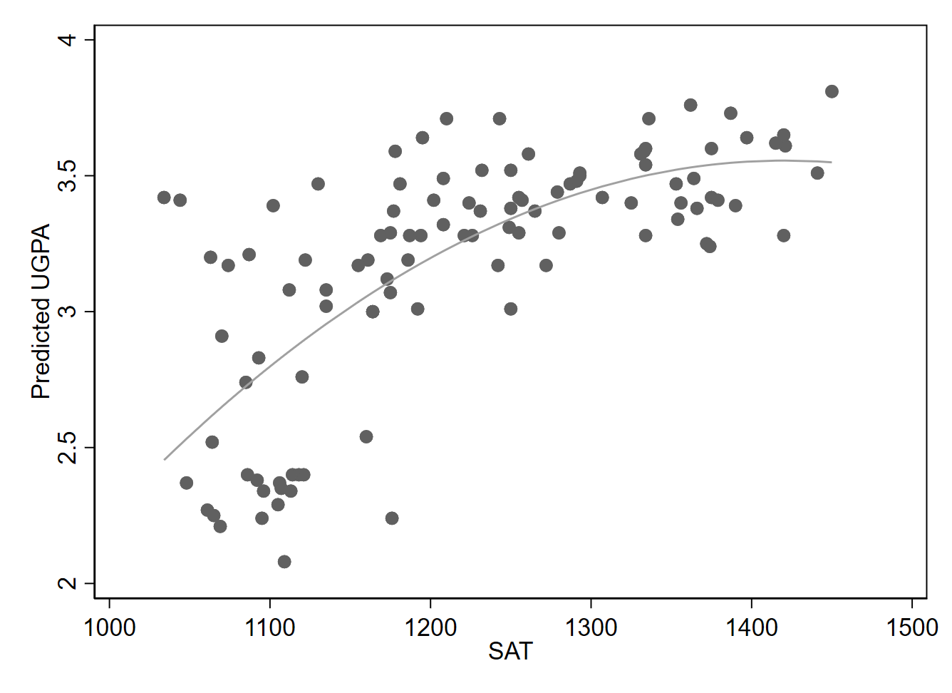
One way to model a non-linear relationship is to square the values of an independent variable, and then include both the original (non-squared) version of the variable as well as the squared variable in the regression. Doing so with the SAT variable, we find our estimates generate the following equation (with university GPA as the dependent variable):

\[ \widehat{UGPA}_i = -11.331 + 0.021 \times SAT_i - 0.0000074 \times SAT^2_i \]

This results in the curved line shown in Figure 11.2, which better tracks the data in the scatterplot than a straight line would. Adding a squared line allows for the shape of the line to follow the shape of a parabola. If we want to allow for a second bend in the line (of a certain sort), we could add a cubed term. Higher-level polynomials can also be added.

Figure 11.2: Adding a squared term to a regression allows the regression line to curve

Now, let’s consider a moderating relationship, meaning that two independent variable interact such that they each alter the association of the other with the dependent variable. Especially when looking at data that is well-suited for drawing causal conclusions, we might also describe tools for modeling moderation as checking for heterogeneous effects. One of the simplest ways to look for potential moderation is to divide a sample into subsamples according to the value of a moderating variable; we can then estimate the association of the independent and dependent variable in each subsample and see whether results differ notably across subsamples.

Let’s check whether the SAT-UGPA relationship appears to differ depending on the value of high school GPA. We split the sample into two subsamples, with one subsample (the “low HSGPA” subsample) containing all students with a high school GPA at or below the full sample’s median. The other subsample (“high HSGPA”) contains students with a value of high school GPA above the median. Note that there are many different ways we might split the sample, such as using the mean instead of the median, or creating three subsamples (low, medium, high).

Estimating a regression line among our low HSGPA subsample yields a slope of 0.0029:

\[ \widehat{UGPA}_i = -0.448 + 0.0029 \times SAT_i \]

Estimated among students in the high HSGPA subsample, the slope shrinks to just 0.00062:

\[ \widehat{UGPA}_i = 2.663 + 0.00062 \times SAT_i \]

Figure 11.3 shows these two distinct lines, along with the underlying subsamples from which they are estimated.

Figure 11.3: Estimating two regressions separately by subsample

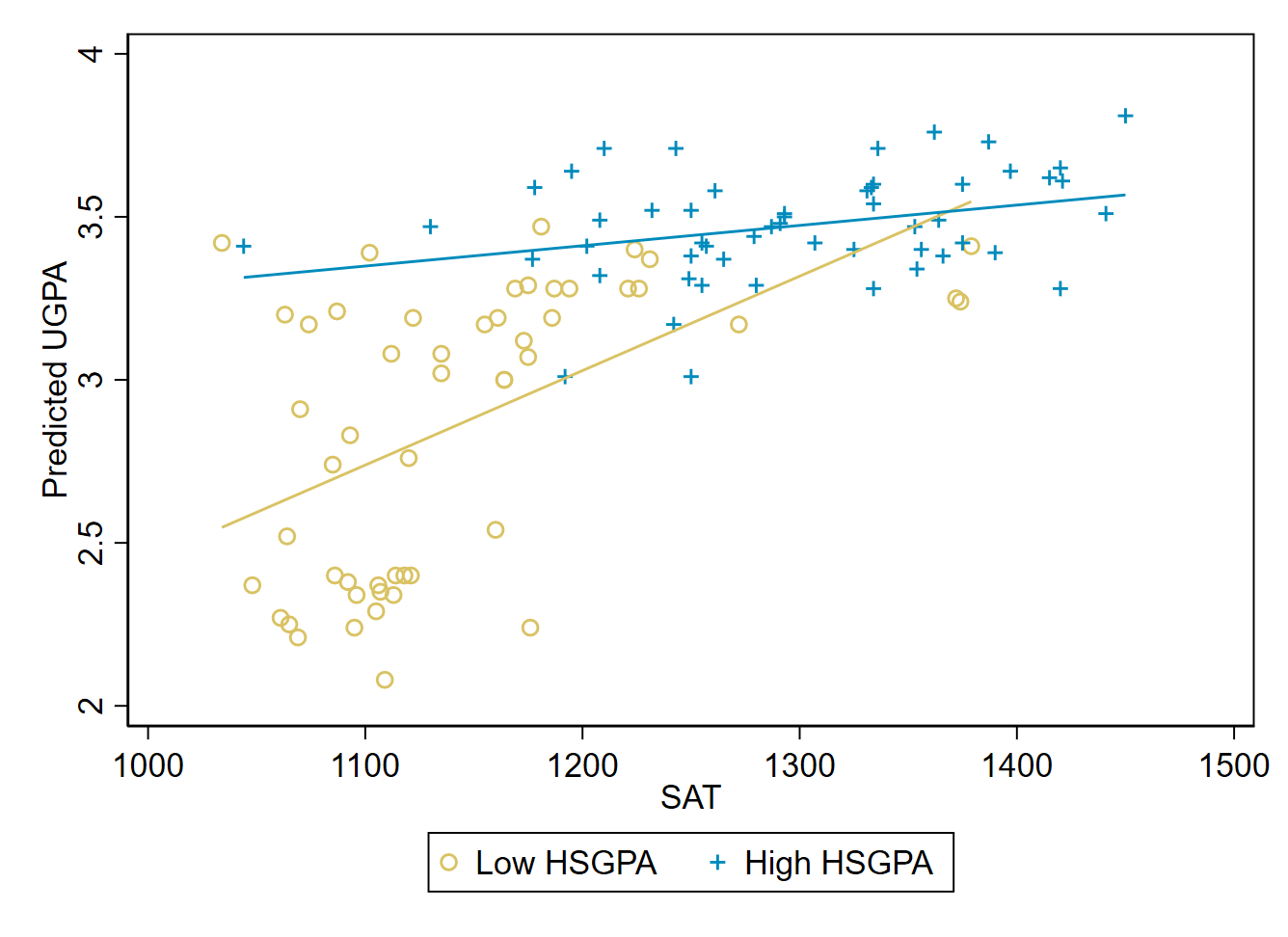
It appears that SAT scores have a stronger association with university GPA (a steeper slope) when high school GPA is low.

We can also model moderation with a single regression for the whole sample using an interaction term. We create an interaction term by multiplying two independent variables together. In this example, we should multiply SAT by high school GPA. We can then run a regression where we have three independent variables: the original SAT variable, the original HSGPA variable, and the interaction term. The regression line is estimated to be:

\[\widehat{UGPA}_i = -3.516 + 1.780 \times HSGPA_i + 0.0043 \times SAT_i - 0.0011 \times HSGPA_i \times SAT_i \]

When we have nonlinear relationships, graphical depictions are typically helpful for demonstrating our results. Using statistical software, we can create a graph that shows us how the predicted value of UGPA changes depending on SAT and certain HSGPA values that we pick out for illustrative purposes. In this case, I chose values of 3.7 (approximately the 90th percentile), 2.3 (approximately the 10th percentile, and 3.0 (half way between the 10th and 90th percentiles).

Figure 11.4: Visualization of a moderating relationship, estimated with an interaction term

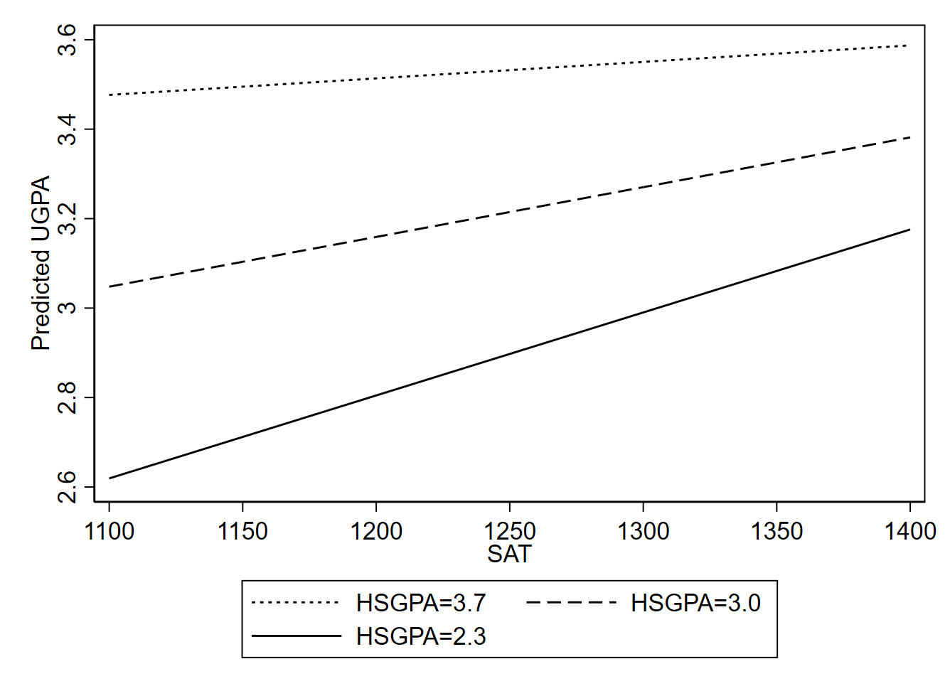
From Figure 11.4, we again see evidence that for higher levels of HSGPA, the relationship of SAT with university GPA gets weaker. However, an important caveat to this finding is that the coefficient for the interaction term is not statistically significant at the traditional .05 alpha level (p=0.069), so there is not strong statistical evidence that the slope does in fact vary depending on HSGPA. In other words, the changes we see in the slope in Figure 11.4 could easily be a coincidence, given the imprecision of our estimate. A larger sample could help us better assess whether the moderating relationship that we seem to observe is more than a statistical anomaly.

More generally, it typically requires a large sample size to generate precise estimates of non-linear relationships.¹¹

While the approaches described in this section are widely employed in the social sciences, caution is warranted whenever modeling non-linearities with quantitative independent variables (interaction effects involving one or more binary independent variables are more straightforward to work with). Adding interaction or polynomial terms to linear regression equations is a somewhat inflexible way of dealing with potential non-linearities; we can easily go wrong if there are relatively small deviations from the functional form we assume in the regression equation we choose to use for our model. Put differently, it is hard to be confidence we are not violating regression assumptions 1 and 3 in a consequential way when relying on these simplistic methods to describe the details of a non-linear relationship. Fortunately, it is not too difficult to find more flexible approaches that can help validate findings of non-linearities in which we are interested, although doing so may require learning tools (e.g., nonparametric regression) beyond the scope of what is covered in this text.¹²

11.4 Exercises

1. Suppose I want to predict country crime rates based on income inequality, gun ownership rates, and ethnoracial heterogeneity. Write out a linear regression equation that allows for this type of prediction.
2. If I want to control for Z (another variable) in my estimation of the effect of X on Y, how do I set up my regression?
3. Suppose you want to understand how a prison education program affects prisoners. You argue that those who participate in the program are likely to experience increased self-efficacy (a sense of confidence that they can achieve their goals). And you think that those with higher self-efficacy will be less likely to recidivate (commit another crime after being released from prison). In sum, you expect participation in the education program to reduce recidivism by increasing self-efficacy. What are your independent, dependent, and mediating variables?
4. Based on the argument outlined in the prior question, write 3 hypotheses describing your expectations for how the three variables are related to one another. Each hypothesis should describe what sort of correlation (positive or negative) you expect there to be between two variables (e.g., A is positively related to B).

Chapter 11 Appendix: More Explanation of Partial Slopes/Associations

The simple linear regression equation can be written as:

\[ \hat{y_i} = \alpha + \beta x_i \tag{11.3}\]

We estimate the value of the slope coefficient (using least squares) as:

\[ \hat{\beta} = \frac{Cov(x,y)}{Var(x)} \tag{11.4}\]

When we have two independent variables (x and z), the corresponding equations are:

\[ \hat{y_i} = \alpha + \beta_1 x_i + \beta_2 z_i \tag{11.5}\]

\[ \hat{\beta_1} = \frac{ Cov(x,y) Var(z) - Cov(z,y) Cov(x,z) } {Var(x) Var(z) - Cov(x,z)^2 } \tag{11.6}\]

Notice that in the numerator of Equation 11.6, we begin with the covariance between x and y (which we also scale by multiplying by the variance of z). Then, to avoid a spurious relationship between x and y that might stem from z affecting both x and y, we subtract out the covariance of z and y times the covariance of z and x. Conceptually, we throw out the joint variation among all three variables—the portion of the overlap between x and y that also reflects overlap between z and y and between z and x.

One way to think about the partial associations obtained through multiple regression is to use a Venn diagram to illustrate how covariance among three (or more) variables is handled.¹³ This is not a perfectly precise representation of how multiple regression works, but it can serve as a helpful tool for understanding the basic intuition. Think of overlap in circles as representing common variation or covariation.

Figure 11.5

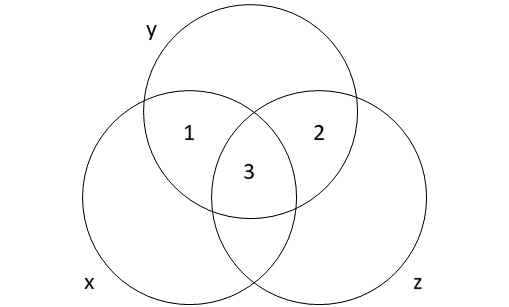
When estimating partial slopes (multiple regression), the coefficient estimate for x is based on area 1. The coefficient estimate for z is based on area 2. Shared variation among all variables can’t be easily attributed to x or z, so area 3 isn’t be used to estimate either coefficient in multiple regression. If we estimate the coefficient of x using simple linear regression (without including z in the regression model), we might get a misleading estimate of the relationship between x and y since we’ll be using areas 1 and 3 to estimate the coefficient for x. If z is a confounding variable, then including area 3 when estimating a slope for x may be undesirable since this portion of the covariation between x and y is due to a common cause (z) rather than a direct link between x and y.

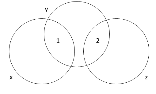
But what about when the two independent variables x and z are uncorrelated? If the covariance between them is zero, then their variation is already independent (at least linearly independent). And therefore, finding the independent association of each one with y is equivalent to just finding the association with y. Using the Ballantine visual, there is no overlapping part 3 to subtract out, as seen in Figure 11.6.

Figure 11.6

Looking to Equation 11.6, we can try subbing in the value 0 for \(Cov(x,z)\):

\[ \hat{\beta_1} = \frac{ Cov(x,y) Var(z) - Cov(z,y) (0) } {Var(x) Var(z) - (0)^2 } \]\[ = \frac{ Cov(x,y) Var(z) } {Var(x) Var(z) } = \frac{ Cov(x,y) } {Var(x) }\]

This yields the same result as Equation 11.4, indicating that we obtain the same slope coefficient estimate for x regardless of whether we use simple regression or control for z in the case where x and z are perfectly uncorrelated. Note that this result only applies to the slope’s point estimate; its standard error and confidence interval will likely differ.

We can also use the language of conditional expected values to demonstrate the difference between the bivariate (zero-order) associations described by simple regression and the partial associations found in multiple regression. Regression can be conceptualized as a model of a conditional expected value (conditional mean), where the predicted value (for the dependent variable) is an expected value and we are conditioning on the independent variables in the regression.

Returning to the example from Section 11.2, we can indicate the difference in expected university GPA between two students where the only thing we know about them is that one (student A) has a high school GPA of 3.5 and the other (student B) has a high school GPA of 2.5. If high school GPA is the only piece of information we have access to, we should use the simple linear regression Equation 11.2 to determine this expected difference:

\[ \mathbb{E}[UGPA|HSGPA=3.5]-\mathbb{E}[UGPA|HSGPA=2.5] \]\[ = [1.097 + 0.675 \times (3.5)] - [1.097 + 0.675 \times (2.5)] = 0.675 \]

Now, suppose that we also know the two students’ SAT scores. If they are both 1100, that changes the predictive effect of a 1-point difference in high school GPA because would would have guessed that student A (with the 3.5 high school GPA) had a higher SAT score than student B (with a 2.5 high school GPA) since these two variables are positively correlated. But with partial slopes, we are considering how changing the value of one variable alters our prediction while holding all other variables constant. The partial slope for \(HSGPA\) in Equation 11.1 indicates the difference in the expected value of university GPA when the \(HSGPA\) differ by one but the SAT scores are equal:

\[\mathbb{E}[UGPA|HSGPA=3.5, SAT=1100]-\mathbb{E}[UGPA|HSGPA=2.5, SAT=1100] \]\[ =[0.540 + 0.541 \times (3.5) + 0.008 \times (1100)] - [0.540 + 0.541 \times (2.5) + 0.008 \times (1100)] \]\[ = 0.541\]

The key point to emphasize here is that the difference in the expected value of university GPA associated with a 1-point difference in high school GPA changes depending on whether we are conditioning on solely high school GPA (yielding a difference of 0.675) or if we are also conditioning on SAT (yielding a difference of 0.541). That is because holding SAT constant is not what we would normally expect when observing a difference in high school GPA, since high school GPA and SAT are (positively) correlated.

---

1. One way to conceptualize potential consequences of violating of this assumption is that you are effectively overstating the sample size: since observations are not truly independent, each observation adds less than a full unit (of new information) to the degrees of freedom.

2. Some additional techniques beyond those mentioned in the main text are spatial regression models, time series and panel regression techniques, and fixed effects models.

3. Take, for example, a study of whether employee job satisfaction is associated with changes in the size of an organization’s budget. Suppose a survey is conducted with employees of several dozen organizations, yielding thousands of individual-level survey responses. This seems to provide a very large sample, but the independent variable—size of the organization’s budget—is measured at the level of the organization, not at the level of the individual. And only a few dozen organizations were included in the sample. This is a classic example of multi-level data (since job satisfaction is measured at the individual level while budget size is measured at the organizational level). With multi-level data, it is difficult to define the sample size because the sample size differs depending on the variable: individual-level variables will have many more distinct observations than organizational-level variables. If we run a regression at the individual level, we risk dramatically overstating the precision of our estimates due to acting as though our sample size is much larger than it really is (for the independent variable).

4. The first paragraph of this subsection is adapted from David M. Lane. “Inferential Statistics for b and r.” Online Statistics Education: A Multimedia Course of Study. https://onlinestatbook.com/2/regression/inferent

5. Rajh-Weber, H., Huber, S.E. & Arendasy, M. A practice-oriented guide to statistical inference in linear modeling for non-normal or heteroskedastic error distributions. Behav Res 57, 338 (2025). https://doi.org/10.3758/s13428-025-02801-4

6. Field, A. P., & Wilcox, R. R. (2017). Robust statistical methods: A primer for clinical psychology and experimental psychopathology researchers. Behaviour research and therapy, 98, 19-38. https://doi.org/10.1016/j.brat.2017.05.013

   Baissa, D. K., & Rainey, C. (2020). When BLUE is not best: non-normal errors and the linear model. Political Science Research and Methods, 8(1), 136-148. https://doi.org/10.1017/psrm.2018.34

7. The initial material in this section (up until Section 11.2.1) is adapted from Rudy Guerra and David M. Lane. “Introduction to Multiple Regression.” Online Statistics Education: A Multimedia Course of Study. https://onlinestatbook.com/2/regression/multiple_regression.html

8. A linear combination of variables is a way of creating a new variable by combining other variables. A linear combination is one in which each variable is multiplied by a coefficient and the products are summed. For example, if
   \[y_i = 3x_{1i} + 2x_{2i} + .5x_{3i}\]
   then \(y\) is a linear combination of the variables \(x_1\), \(x_2\), and \(x_3\).

9. The remainder of the chapter was written by Nathan Favero.

10. Green, D. P., Ha, S. E., & Bullock, J. G. (2010). Enough already about “black box” experiments: Studying mediation is more difficult than most scholars suppose. The Annals of the American Academy of Political and Social Science, 628(1), 200-208.

11. It is difficult to say precisesly how large, but see the following resources for more concrete guidance:

    Gelman, A. (2018). You need 16 times the sample size to estimate an interaction than to estimate a main effect [blog post]. https://statmodeling.stat.columbia.edu/2018/03/15/need16/

    Sommet, N., et al. (2023). How many participants do I need to test an interaction? Conducting an appropriate power analysis and achieving sufficient power to detect an interaction. Advances in Methods and Practices in Psychological Science, 6(3), 25152459231178728.

    Baranger, D. A., et al. (2023). Tutorial: Power analyses for interaction effects in cross-sectional regressions. Advances in Methods and Practices in Psychological Science, 6(3), 25152459231187531.

12. Simonsohn U. Interacting With Curves: How to Validly Test and Probe Interactions in the Real (Nonlinear) World. Advances in Methods and Practices in Psychological Science. 2024;7(1). doi:10.1177/25152459231207787

    Hainmueller, J., Mummolo, J., & Xu, Y. (2019). How much should we trust estimates from multiplicative interaction models? Simple tools to improve empirical practice. Political Analysis, 27(2), 163-192. https://doi.org/10.1017/pan.2018.46

    Simonsohn U. Two Lines: A Valid Alternative to the Invalid Testing of U-Shaped Relationships With Quadratic Regressions. Advances in Methods and Practices in Psychological Science. 2018;1(4):538-555. doi:10.1177/2515245918805755

13. Kennedy (2002) and Cohen and Cohen (1975) have been instrumental in developing this Ballentine diagram approach to explaining multiple regression.

    Kennedy, P. (2008). A guide to econometrics. Malden, MA: Blackwell Publishing.

    Cohen, J., & Cohen, P. (1975). Applied Multiple Regression/Correlation Analysis for the Behavioral Sciences. Hillsdale, NJ: Lawrence Erlbaum Associates.